In my last post I mapped out how one could test the reliability of a single stock strategy (for the S&P 500 Index) using synthetic data generated by the new algorithm I developed.
As this piece of research follows a similar path, I won’t repeat all those details here. The key point addressed in this post is that not only are we able to generate consistent open/high/low/close prices for individual stocks, we can do so in a way that preserves the correlations between related securities. In other words, the algorithm not only replicates the time series properties of individual stocks, but also the cross-sectional relationships between them. This has important applications for the development of portfolio strategies and portfolio risk management.
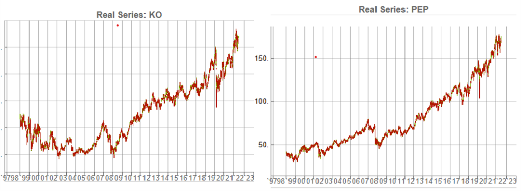
KO-PEP Pair
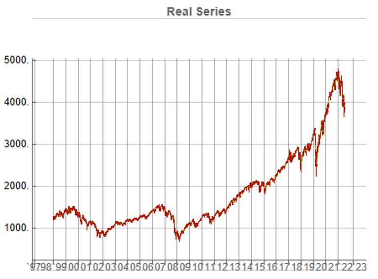
To illustrate this I will use synthetic daily data to develop a pairs trading strategy for the KO-PEP pair.
The two price series are highly correlated, which potentially makes them a suitable candidate for a pairs trading strategy.
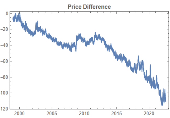
There are numerous ways to trade a pairs spread such as dollar neutral or beta neutral, but in this example I am simply going to look at trading the price difference. This is not a true market neutral approach, nor is the price difference reliably stationary. However, it will serve the purpose of illustrating the methodology.
Historical price differences between KO and PEP
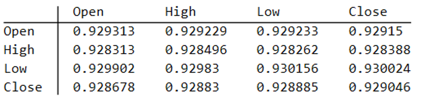
Obviously it is crucial that the synthetic series we create behave in a way that replicates the relationship between the two stocks, so that we can use it for strategy development and testing. Ideally we would like to see high correlations between the synthetic and original price series as well as between the pairs of synthetic price data.
We begin by using the algorithm to generate 100 synthetic daily price series for KO and PEP and examine their properties.
Correlations
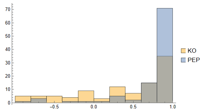
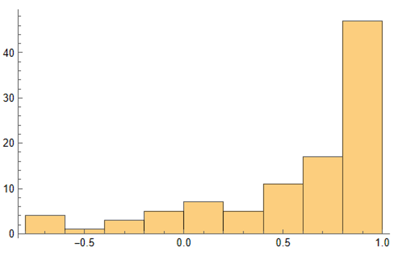
As we saw previously, the algorithm is able to generate synthetic data with correlations to the real price series ranging from below zero to close to 1.0:
Distribution of correlations between synthetic and real price series for KO and PEP
The crucial point, however, is that the algorithm has been designed to also preserve the cross-sectional correlation between the pairs of synthetic KO-PEP data, just as in the real data series:
Distribution of correlations between synthetic KO and PEP price series
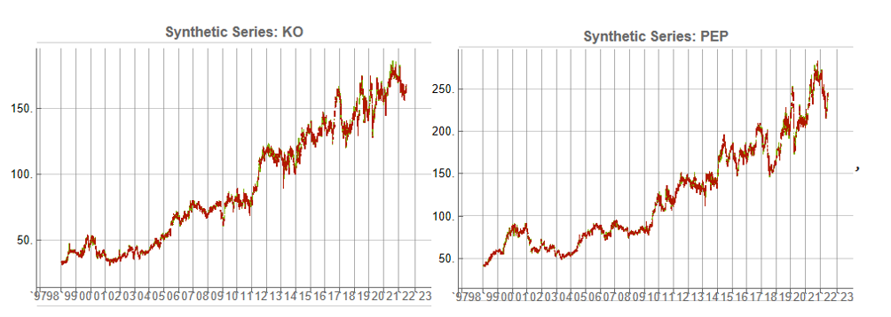
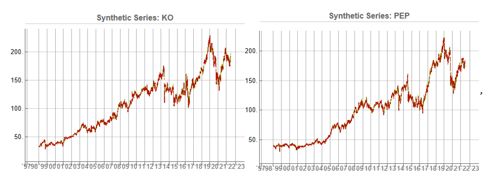
Some examples of highly correlated pairs of synthetic data are shown in the plots below:
In addition to correlation, we might also want to consider the price differences between the pairs of synthetic series, since the strategy will be trading that price difference, in the simple approach adopted here. We could, for example, select synthetic pairs for which the divergence in the price difference does not become too large, on the assumption that the series difference is stationary. While that approach might well be reasonable in other situations, here an assumption of stationarity would be perhaps closer to wishful thinking than reality. Instead we can use of selection of synthetic pairs with high levels of cross-correlation, as we all high levels of correlation with the real price data. We can also select for high correlation between the price differences for the real and synthetic price series.
Strategy Development& WFO Testing
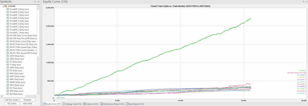
Once again we follow the procedure for strategy development outline in the previous post, except that, in addition to a selection of synthetic price difference series we also include 14-day correlations between the pairs. We use synthetic daily synthetic data from 1999 to 2012 to build the strategy and use the data from 2013 onwards for testing/validation. Eventually, after 50 generations we arrive at the result shown in the figure below:
As before, the equity curve for the individual synthetic pairs are shown towards the bottom of the chart, while the aggregate equity curve, which is a composition of the results for all none synthetic pairs is shown above in green. Clearly the results appear encouraging.
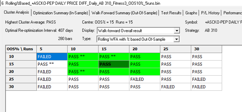
As a final step we apply the WFO analysis procedure described in the previous post to test the performance of the strategy on the real data series, using a variable number in-sample and out-of-sample periods of differing size. The results of the WFO cluster test are as follows:
The results are no so unequivocal as for the strategy developed for the S&P 500 index, but would nonethless be regarded as acceptable, since the strategy passes the great majority of the tests (in addition to the tests on synthetic pairs data).
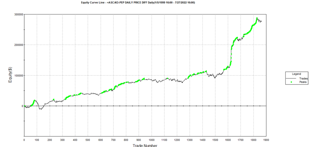
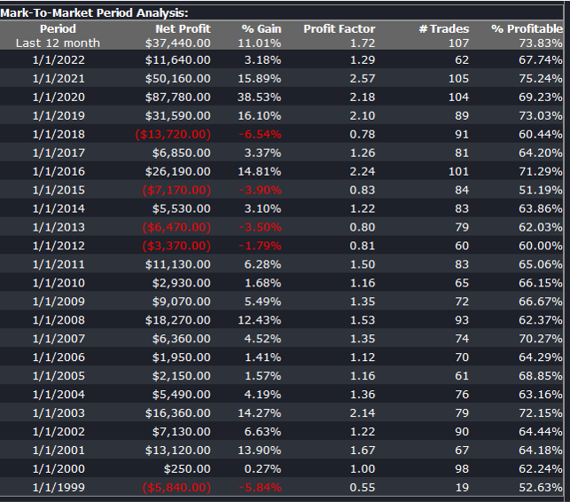
The final results appear as follows:
Conclusion
We have demonstrated how the algorithm can be used to generate synthetic price series the preserve not only the important time series properties, but also the cross-sectional properties between series for correlated securities. This important feature has applications in the development of statistical arbitrage strategies, portfolio construction methodology and in portfolio risk management.
One of the main criticisms levelled at systematic trading over the last few years is that the over-use of historical market data has tended to produce curve-fitted strategies that perform poorly out of sample in a live trading environment. This is indeed a valid criticism – given enough attempts one is bound to arrive eventually at a strategy that performs well in backtest, even on a holdout data sample. But that by no means guarantees that the strategy will continue to perform well going forward.
The solution to the problem has been clear for some time: what is required is a method of producing synthetic market data that can be used to build a strategy and test it under a wide variety of simulated market conditions. A strategy built in this way is more likely to survive the challenge of live trading than one that has been developed using only a single historical data path.
The problem, however, has been in implementation. Up until now all the attempts to produce credible synthetic price data have failed, for one reason or another, as I described in an earlier post:
I have been able to devise a completely new algorithm for generating artificial price series that meet all of the key requirements, as follows:
Computational simplicity & efficiency. Important if we are looking to mass-produce synthetic series for a large number of assets, for a variety of different applications. Some deep learning methods would struggle to meet this requirement, even supposing that transfer learning is possible.
The ability to produce price series that are internally consistent (i.e High > Low, etc) in every case .
Should be able to produce a range of synthetic series that vary widely in their correspondence to the original price series. In some case we want synthetic price series that are highly correlated to the original; in other cases we might want to test our investment portfolio or risk control systems under extreme conditions never before seen in the market.
The distribution of returns in the synthetic series should closely match the historical series, being non-Gaussian and with “fat-tails”.
The ability to incorporate long memory effects in the sequence of returns.
The ability to model GARCH effects in the returns process.
This means that we are now in a position to develop trading strategies without any direct reference to the underlying market data. Consequently we can then use all of the real market data for out-of-sample back-testing.
Developing a Trading Strategy for the S&P 500 Index Using Synthetic Market Data
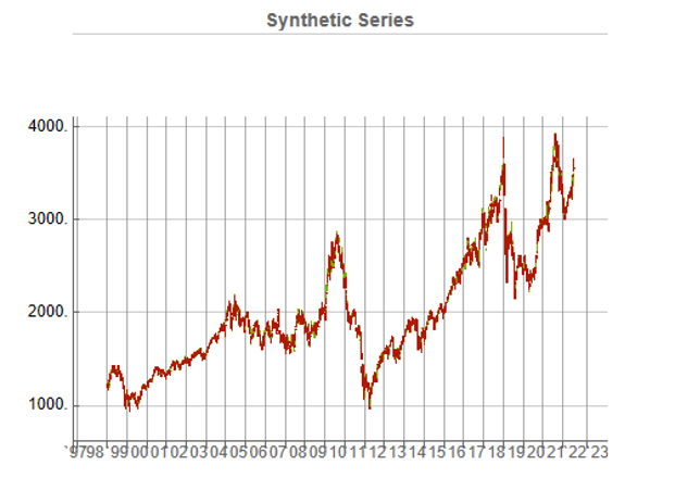
To illustrate the procedure I am going to use daily synthetic price data for the S&P 500 Index over the period from Jan 1999 to July 2022. Details of the the characteristics of the synthetic series are given in the post referred to above.
Because we want to create a trading strategy that will perform under market conditions close to those currently prevailing, I will downsample the synthetic series to include only those that correlate quite closely, i.e. with a minimum correlation of 0.75, with the real price data.
Why do this? Surely if we want to make a strategy as robust as possible we should use all of the synthetic data series for model development?
The reason is that I believe that some of the more extreme adverse scenarios generated by the algorithm may occur quite rarely, perhaps once in every few decades. However, I am principally interested in a strategy that I can apply under current market conditions and I am prepared to take my chances that the worst-case scenarios are unlikely to come about any time soon. This is a major design decision, one that you may disagree with. Of course, one could make use of every available synthetic data series in the development of the trading model and by doing so it is likely that you would produce a model that is more robust. But the training could take longer and the performance during normal market conditions may not be as good.
Having generated the price series, the process I am going to follow is to use genetic programming to develop trading strategies that will be evaluated on all of the synthetic data series simultaneously. I will then use the performance of the aggregate portfolio, i.e. the outcome of all of the trades generated by the strategy when applied to all of the synthetic series, to assess the overall performance. In order to be considered, candidate strategies have to perform well under all of the different market scenarios, or at least the great majority of them. This ensures that the strategy is likely to prove more robust across different types of market conditions, rather than on just the single type of market scenario observed in the real historical series.
As usual in these cases I will reserve a portion (10%) of each data series for testing each strategy, and a further 10% sample for out-of-sample validation. This isn’t strictly necessary: since the real data series has not be used directly in the development of the trading system, we can later test the strategy on all of the historical data and regard this as an out-of-sample backtest.
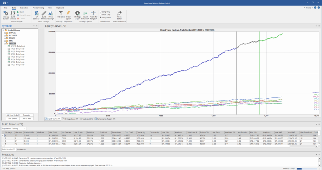
To implement the procedure I am going to use Mike Bryant’s excellent Adaptrade Builder software.
This is an exemplar of outstanding software engineering and provides a broad range of features for generating trading strategies of every kind. One feature of Builder that is particularly useful in this context is its ability to construct strategies and test them on up to 20 data series concurrently. This enables us to develop a strategy using all of the synthetic data series simultaneously, showing the performance of each individual strategy as well for as the aggregate portfolio.
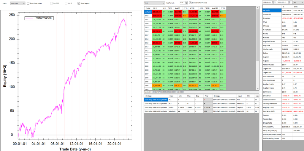
After evolving strategies for 50 generations we arrive at the following outcome:
The equity curve for the aggregate portfolio is shown in blue, while the equity curves for the strategy applied to individual synthetic data series are shown towards the bottom of the chart. Of course, the performance of the aggregate portfolio appears much superior to any of the individual strategies, because it is effectively the arithmetic sum of the individual equity curves. And just because the aggregate portfolio appears to perform well both in-sample and out-of-sample, that doesn’t imply that the strategy works equally well for every individual market scenario. In some scenarios it performs better than in others, as can be observed from the individual equity curves.
But, in any case, our objective here is not to create a stock portfolio strategy, but rather to trade a single asset – the S&P 500 Index. The role of the aggregate portfolio is simply to suggest that we may have found a strategy that is sufficiently robust to work well across a variety of market conditions, as represented by the various synthetic price series.
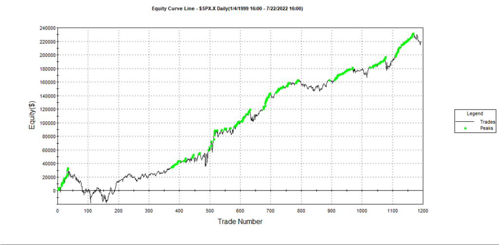
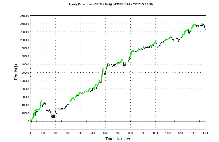
Builder generates code for the strategies it evolves in a number of different languages and in this case we take the EasyLanguage code for the fittest strategy #77 and apply it to a daily chart for the S&P 500 Index – i.e. the real data series – in Tradestation, with the following results:
The strategy appears to work well “out-of-the-box”, i,e, without any further refinement. So our quest for a robust strategy appears to have been quite successful, given that none of the 23-year span of real market data on which the strategy was tested was used in the development process.
We can take the process a little further, however, by “optimizing” the strategy. Traditionally this would mean finding the optimal set of parameters that produces the highest net profit on the test data. But this would be curve fitting in the worst possible sense, and is not at all what I am suggesting.
Instead we use a procedure known as Walk Forward Optimization (WFO), as described in this post:
The goal of WFO is not to curve-fit the best parameters, which would entirely defeat the object of using synthetic data. Instead, its purpose is to test the robustness of the strategy. We accomplish this by using a sequence of overlapping in-sample and out-of-sample periods to evaluate how well the strategy stands up, assuming the parameters are optimized on in-sample periods of varying size and start date and tested of similarly varying out-of-sample periods. A strategy that fails a cluster of such tests is unlikely to prove robust in live trading. A strategy that passes a test cluster at least demonstrates some capability to perform well in different market regimes.
To some extent we might regard such a test as unnecessary, given that the strategy has already been observed to perform well under several different market conditions, encapsulated in the different synthetic price series, in addition to the real historical price series. Nonetheless, we conduct a WFO cluster test to further evaluate the robustness of the strategy.
As the goal of the procedure is not to maximize the theoretical profitability of the strategy, but rather to evaluate its robustness, we select a criterion other than net profit as the factor to optimize. Specifically, we select the sum of the areas of the strategy drawdowns as the quantity to minimize (by maximizing the inverse of the sum of drawdown areas, which amounts to the same thing). This requires a little explanation.
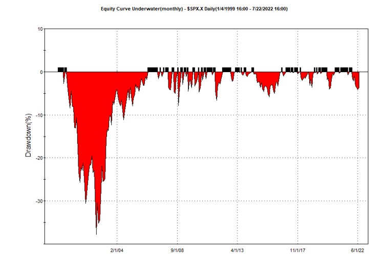
If we look at the strategy drawdown periods of the equity curve, we observe several periods (highlighted in red) in which the strategy was underwater:
The area of each drawdown represents the length and magnitude of the drawdown and our goal here is to minimize the sum of these areas, so that we reduce both the total duration and severity of strategy drawdowns.
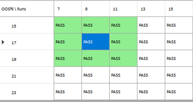
In each WFO test we use different % of OOS data and a different number of runs, assessing the performance of the strategy on a battery of different criteria:
x
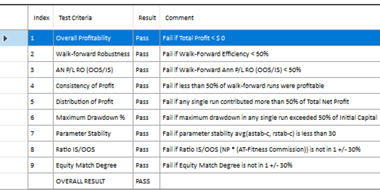
These criteria not only include overall profitability, but also factors such as parameter stability, profit consistency in each test, the ratio of in-sample to out-of-sample profits, etc. In other words, this WFO cluster analysis is not about profit maximization, but robustness evaluation, as assessed by these several different metrics. And in this case the strategy passes every test with flying colors:
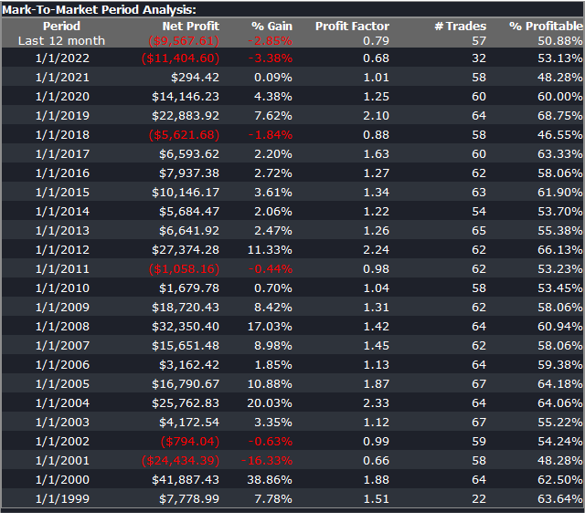
Other than validating the robustness of the strategy’s performance, the overall effect of the procedure is to slightly improve the equity curve by diminishing the magnitude and duration of the drawdown periods:
Conclusion
We have shown how, by using synthetic price series, we can build a robust trading strategy that performs well under a variety of different market conditions, including on previously “unseen” historical market data. Further analysis using cluster WFO tests strengthens the assessment of the strategy’s robustness.
Momentum trading strategies span a diverse range of trading ideas. Often they will use indicators to determine the recent underlying trend and try to gauge the strength of the trend using measures of the rate of change in the price of the asset.
One very simple momentum concept, a strategy in S&P500 E-Mini futures, is described in the following blog post:
The basic idea is to buy the S&P500 E-Mini futures when the contract makes a new intraday high. This is subject to the qualification that the Internal Bar Strength fall below a selected threshold level. In order words, after a period of short-term weakness – indicated by the low reading of the Internal Bar Strength – we buy when the futures recover to make a new intraday high, suggesting continued forward momentum.
IBS is quite a useful trading indicator, which you can learn more about in these posts:
I have developed a version of the intraday-high strategy, using parameters to generalize it and allow for strategy optimization. The Easylanguage code for my version of the strategy is as follows:
If H[IBSlag] > L[IBSlag] then
Begin
IBS=(H[IBSlag]-C[IBSlag])/(H[IBSlag]-L[IBSlag]);
end;
If (IBS <= IBStrigger) and (H[0] >= Highest(High, ndaysHigh)) then
begin
Buy nContracts contracts this bar on close;
end;
If C[0] > H[1] then
begin
Sell all contracts this bar on close;
end;
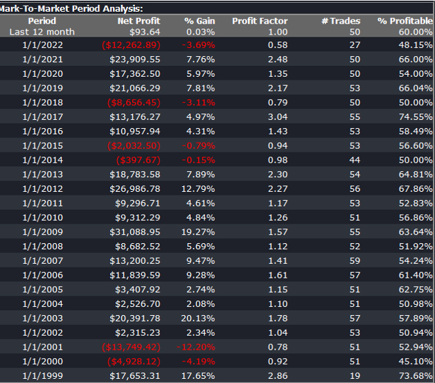
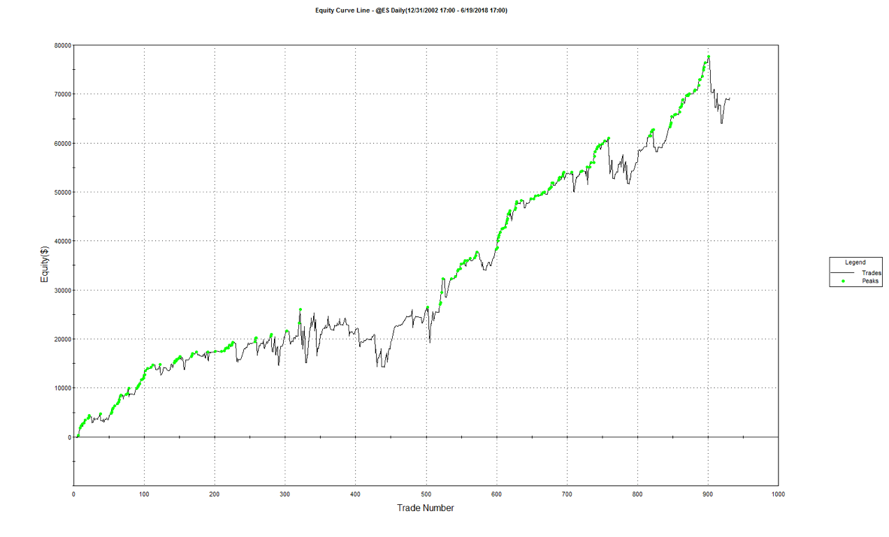
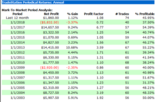
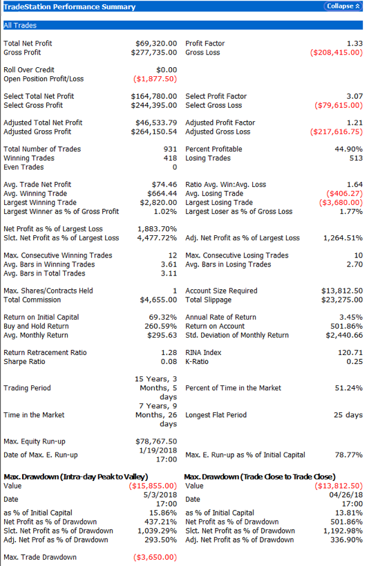
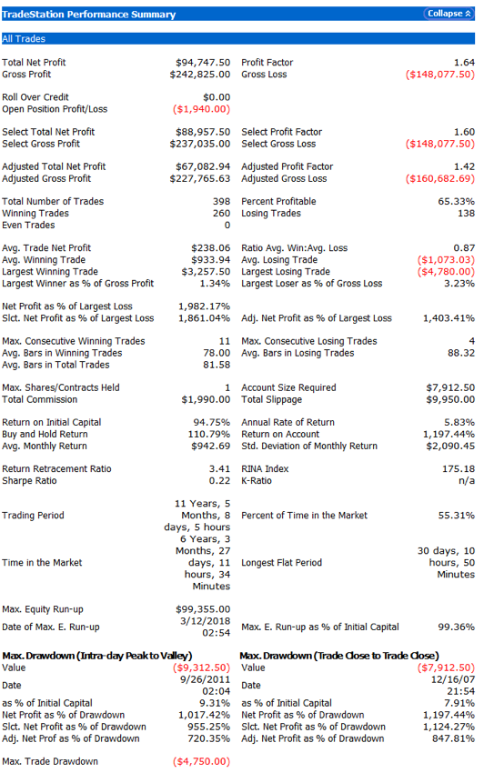
The performance results for the strategy appear quite promising, despite the downturn in strategy profitability in 2018 to date (all performance results are net of slippage and commission):
Robustness Testing with Walk Forward Optimization
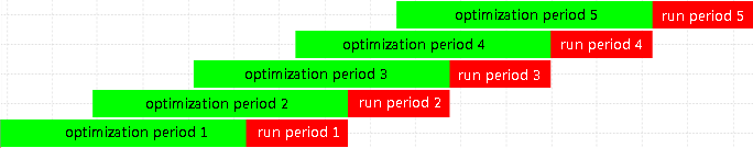
We evaluate the robustness of the strategy using the Walk Forward Optimization feature in Tradestation. Walk forward analysis is the process of optimizing a trading system using a limited set of parameters, and then testing the best optimized parameter set on out-of-sample data. This process is similar to how a trader would use an automated trading system in real live trading. The in-sample time window is shifted forward by the period covered by the out-of-sample test, and the process is repeated. At the end of the test, all of the recorded results are used to assess the trading strategy.
In other words, walk forward analysis does optimization on a training set; tests on a period after the set and then rolls it all forward and repeats the process. This gives a larger out-of-sample period and allows the system developer to see how stable the system is over time.
The image below illustrates the walk forward analysis procedure. An optimization is performed over a longer period (the in-sample data), and then the optimized parameter set is tested over a subsequent shorter period (the out-of-sample data). The optimization and testing periods are shifted forward, and the process is repeated until a suitable sample size is achieved.
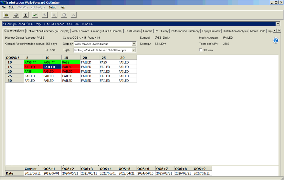
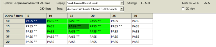
Tradestation enables the user to run a battery of WFO tests, using different size in-sample and out-of-sample sizes and number of runs. The outcome of each test is evaluated on several specific criteria such as the net profit and drawdown and only if the system meets all of the criteria is the test designated as a “Pass”. This gives the analyst a clear sense of the robustness of his strategy across multiple periods and sample sizes.
A WFO cluster analysis summary for the momentum strategy is illustrated below. The cluster test is designated as “Failed” overall, since the strategy failed to meet the test criteria for a preponderance of the individual walk-forward tests. The optimal parameters found in each test vary considerably over the sample periods spanning 2003-2018, giving concerns about the robustness of the strategy under changing market conditions.
Improving the Strategy
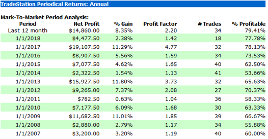
We can improve both the performance and robustness of our simple momentum strategy by combining it with several other trend and momentum indicators. One such example is illustrated in the performance charts and tables below. The strategy has performed well in both bull and bear markets and in both normal and volatile market conditions:
A WFO cluster analysis indicates that the revised momentum strategy is highly robust to the choice of sample size and strategy parameters, as it passes every test in the 30-cell WFO analysis cluster table:
Conclusion
Momentum strategies are well known and easy to develop using standard methodologies, such as the simple indicators used in this example. They tend to work well in most equity index futures markets, and in some commodity markets too. One of their big drawbacks, however, is that they typically go through periods of poor performance and need to be tested thoroughly for robustness in order to ensure satisfactory results under the full range of market conditions.