State-Space Models for Market Microstructure: Can Mamba Replace Transformers in High-Frequency Finance?

In my recent piece on Kronos, I explored how foundation models trained on K-line data are reshaping time series forecasting in finance. That discussion naturally raises a follow-up question that several readers have asked: what about the architecture itself? The Transformer has dominated deep learning for sequence modeling over the past seven years, but a new class of models — State-Space Models (SSMs), particularly the Mamba architecture — is gaining serious attention. In high-frequency trading, where computational efficiency and latency are everything, the claimed O(n) versus O(n²) complexity advantage is more than academic. It’s a potential competitive edge.

Let me be clear from the outset: I’m skeptical of any claim that a new architecture will “replace” Transformers wholesale. The Transformer ecosystem is mature, well-understood, and backed by enormous engineering investment. But in the specific context of market microstructure — where we process millions of tick events, model limit order book dynamics, and make decisions in microseconds — SSMs deserve serious examination. The question isn’t whether they can replace Transformers entirely, but whether they should be part of our toolkit for certain problems.

I’ve spent the better part of two decades building trading systems that push against latency constraints. I’ve watched the industry evolve from simple linear models to gradient boosted trees to deep learning, each wave promising revolutionary improvements. Most delivered incremental gains; some fizzled entirely. What’s interesting about SSMs isn’t the theoretical promise — we’ve seen theoretical promises before — but rather the practical characteristics that might actually matter in a production trading environment. The linear scaling, the constant-time inference, the selective attention mechanism — these aren’t just academic curiosities. They’re the exact properties that could determine whether a model makes it into a production system or dies in a research notebook.

What Are State-Space Models?

To understand why SSMs have suddenly become interesting, we need to go back to the mathematical foundations — and they’re older than you might think. State-space models originated in control theory and signal processing, describing systems where an internal state evolves over time according to differential equations, with observations emitted from that state. If you’ve used a Kalman filter — and in quant finance, many of us have — you’ve already worked with a simple state-space model, even if you didn’t call it that.

The canonical continuous-time formulation is:

\[x'(t) = Ax(t) + Bu(t)\]

\[y(t) = Cx(t) + Du(t)\]

where $x(t)$ is the latent state vector, $u(t)$ is the input, $y(t)$ is the output, and $A$, $B$, $C$, $D$ are learned matrices. This looks remarkably like a Kalman filter — because it is, in essence, a nonlinear generalization of linear state estimation. The key difference from traditional time series models is that we’re learning the dynamics directly from data rather than specifying them parametrically. Instead of assuming variance follows a GARCH(1,1) process, we let the model discover what the underlying state evolution looks like.

The challenge, historically, was that computing these models was intractable for long sequences. The recurrent view requires iterating through each timestep sequentially; the convolutional view requires computing full convolutions that scale poorly. This is where the S4 model (Structured State Space Sequence) changed the game.

S4, introduced by Gu, Dao et al. (2022), brought three critical innovations. First, it used the HiPPO (High-order Polynomial Projection Operator) framework to initialize the state matrix $A$ in a way that preserves long-range dependencies. Without proper initialization, SSMs suffer from the same vanishing gradient problems as RNNs. The HiPPO matrix is specifically designed so that when the model views a sequence, it can accurately represent all historical information without exponential decay. In financial terms, this means last month’s market dynamics can influence today’s predictions — something vanilla RNNs struggle with.

Author’s Take: This is the key innovation that makes SSMs viable for finance. Without HiPPO, you’d face the same vanishing-gradient failure mode that killed RNN research for decades. The HiPPO initialization is essentially a “warm start” that encodes the mathematical insight that recent history matters more than distant history — but distant history still matters. This is perfectly aligned with how financial markets work: last quarter’s regime still influences pricing, even if less than yesterday’s moves.

HiPPO provides a theoretically grounded initialization that allows the model to remember information from thousands of timesteps ago — critical for financial time series where last week’s patterns may be relevant to today’s dynamics. The mathematical insight is that HiPPO projects the input onto a basis of orthogonal polynomials, maintaining a compressed representation of the full history. This is conceptually similar to how we’d use PCA for dimensionality reduction, except it’s learned end-to-end as part of the model’s dynamics.

Second, S4 introduced structured parameterizations that enable efficient computation via diagonalization. Rather than storing full $N \times N$ matrices where $N$ is the state dimension, S4 uses structured forms that reduce memory and compute requirements while maintaining expressiveness. The key insight is that the state transition matrix $A$ can be parameterized as a diagonal-plus-low-rank form that enables fast computation via FFT-based convolution. This is what gives S4 its computational advantage over traditional SSMs — the structured form turns the convolution from $O(L^2)$ to $O(L \log L)$.

Third, S4 discretizes the continuous-time model into a discrete-time representation suitable for implementation. The standard approach is zero-order hold (ZOH), which treats the input as constant between timesteps:

\[x_{k} = \bar{A}x_{k-1} + \bar{B}u_k\]

\[y_k = \bar{C}x_k + \bar{D}u_k\]

where $\bar{A} = e^{A\Delta t}$, $\bar{B} = (e^{A\Delta t} – I)A^{-1}B$, and similarly for $\bar{C}$ and $\bar{D}$. The bilinear transform is an alternative that can offer better frequency response in some settings:

Author’s Take: In practice, I’ve found ZOH (zero-order hold) works well for most tick-level data — it’s robust to the high-frequency microstructure noise that dominates at sub-second horizons. Bilinear can help if you’re modeling at longer horizons (minutes to hours) where you care more about capturing trend dynamics than filtering out tick-by-tick noise. This is another example of where domain knowledge beats blind architecture choices.

\[\bar{A} = (I + A\Delta t/2)(I – A\Delta t/2)^{-1}\]

Either way, the discretization bridges continuous-time system theory with discrete-time sequence modeling. The choice of discretization matters for financial applications because different discretization schemes have different frequency characteristics — bilinear transform tends to preserve low-frequency behavior better, which may be important for capturing long-term trends.

Mamba, introduced by Gu and Dao (2023) and winning best paper at ICLR 2024, added a fourth critical innovation: selective state spaces. The core insight is that not all input information is equally relevant at all times. In a financial context, during calm markets, we might want to ignore most order flow noise and focus on price levels; during a news event or volatility spike, we want to attend to everything. Mamba introduces a selection mechanism that allows the model to dynamically weigh which inputs matter:

\[s_t = \text{select}(u_t)\]

\[\bar{B}_t = \text{Linear}_B(s_t)\]

\[\bar{C}_t = \text{Linear}_C(s_t)\]

The select operation is implemented as a learned projection that determines which elements of the input to filter. This is fundamentally different from attention — rather than computing pairwise similarities between all tokens, the model learns a function that decides what information to carry forward. In practice, this means Mamba can learn to “ignore” regime-irrelevant data while attending to regime-critical signals.

This selectivity, combined with an efficient parallel scan algorithm (often called S6), gives Mamba its claimed linear-time inference while maintaining the ability to capture complex dependencies. The complexity comparison is stark: Transformers require $O(L^2)$ attention computations for sequence length $L$, while Mamba processes each token in $O(1)$ time with $O(L)$ total computation. For $L = 10,000$ ticks — a not-unreasonable window for intraday analysis — that’s $10^8$ versus $10^4$ operations per layer. The practical implication is either dramatically faster inference or the ability to process much longer sequences for the same compute budget. On modern GPUs, this translates to milliseconds versus tens of milliseconds for a forward pass — a difference that matters when you’re making hundreds of predictions per second.

Compared to RNNs like LSTMs, SSMs don’t suffer from the same sequential computation bottleneck during training. While LSTMs must process tokens one at a time (true parallelization is limited), SSMs can be computed as convolutions during training, enabling GPU parallelism. During inference, SSMs achieve the constant-time-per-token property that makes them attractive for production deployment. This is the key advantage over LSTMs — you get the sequential processing benefits of RNNs during inference with the parallel training benefits of CNNs.

Why HFT and Market Microstructure?

If you’re building trading systems, you’ve likely noticed that most machine learning approaches to finance treat the problem as either (a) predicting returns at some horizon, or (b) classifying market regimes. Neither approach explicitly models the underlying mechanism that generates prices. Market microstructure does exactly that — it models how orders arrive, how limit order books evolve, how informed traders interact with liquidity providers, and how information gets incorporated into prices. Understanding microstructure isn’t just academic — it’s the foundation of profitable execution and market-making strategies.

The data characteristics of market microstructure create unique challenges that make SSMs potentially attractive:

Scale: A single liquid equity can generate millions of messages per day across bid, ask, and depth levels. Consider a highly traded stock like Tesla or Nvidia during volatile periods — you might see 50-100 messages per second, per instrument. A typical algo trading firm’s data pipeline might ingest 50-100GB of raw tick data daily across their coverage universe. Processing this with Transformer models is expensive. The quadratic attention complexity means that doubling your context length quadruples your compute cost. With SSMs, you double context and roughly double compute — a much friendlier scaling curve. This is particularly important when you’re building models that need to see significant historical context to make predictions.

Non-stationarity: Market microstructure is inherently non-stationary. The dynamics of a limit order book during normal trading differ fundamentally from those during a market open, a regulatory halt, or a volatility auction. At market open, you have a flood of overnight orders, wide spreads, and rapid price discovery. During a halt, trading stops entirely and the book freezes. In volatility auctions, you see large price movements with reduced liquidity. Mamba’s selective mechanism is specifically designed to handle this — the model can learn to “switch off” irrelevant inputs when market conditions change. This is conceptually similar to regime-switching models in econometrics, but learned end-to-end. The model learns when to attend to order flow dynamics and when to ignore them based on learned signals.

Latency constraints: In market-making or latency-sensitive strategies, every microsecond counts. A Transformer processing a 512-token sequence might require 262,144 attention operations. Mamba processes the same sequence in roughly 512 state updates — a 500x reduction in per-token operations. While the constants differ (SSM state dimension adds overhead), the theoretical advantage is substantial. Several practitioners I’ve spoken with report sub-10ms inference times for Mamba models that would be impractical with Transformers at the same context length. For comparison, a typical market-making strategy might have a 100-microsecond latency budget for the entire decision pipeline — inference must be measured in microseconds, not milliseconds.

Long-range dependencies: Consider a statistical arbitrage strategy across 100 stocks. A regulatory announcement at 9:30 AM might affect correlations across the entire universe until midday. Capturing this requires modeling dependencies across thousands of timesteps. The HiPPO initialization in S4 and the selective mechanism in Mamba are specifically designed to maintain information flow over such horizons — something vanilla RNNs struggle with due to gradient decay. In practice, this means you can build models that truly “remember” what happened earlier in the trading session, not just what happened in the last few minutes.

There’s also a subtler point worth mentioning: the order book itself is a form of state. When you look at the bid-ask ladder, you’re seeing a snapshot of accumulated order flow — the current state reflects all historical interactions. SSMs are naturally suited to modeling stateful systems because that’s literally what they are. The latent state $x(t)$ in the state equation can be interpreted as an embedding of the current market state, learned from data rather than specified by theory. This is philosophically aligned with how we think about market microstructure: the order book is a state variable, and the messages are observations that update that state.

Recent Research and Results

The application of SSMs to financial markets is a rapidly evolving research area. Let me survey what’s been published, with appropriate skepticism about early-stage results. The key papers worth noting span both the SSM methodology and the finance-specific applications.

On the methodology side, S4 (Gu, Johnson et al., 2022) established the foundation by demonstrating that structured state spaces could match or exceed Transformers on long-range arena benchmarks while maintaining linear computation. The Mamba paper (Gu and Dao, 2023) pushed further by introducing selective state spaces and achieving state-of-the-art results on language modeling benchmarks — remarkable because it suggested SSMs could compete with Transformers on tasks previously dominated by attention. The follow-up work on Mamba 2 (Dao and Gu, 2024) introduced structured state space duals, further improving efficiency.

On the application side, CryptoMamba (Shi et al., 2025) applied Mamba to Bitcoin price prediction, demonstrating “effective capture of long-range dependencies” in cryptocurrency time series. The authors report competitive performance against LSTM and Transformer baselines on several prediction horizons. The cryptocurrency market, with its 24/7 trading and higher noise-to-signal ratio than traditional equities, provides an interesting test case for SSMs’ ability to handle extreme non-stationarity. The paper’s methodology section shows that Mamba’s selective mechanism successfully learned to filter out noise during calm periods while attending to significant price movements — exactly what we’d hope to see.

MambaStock (Liu et al., 2024) adapted the Mamba architecture specifically for stock prediction, introducing modifications to handle the multi-dimensional nature of financial features (price, volume, technical indicators). The selective scan mechanism was applied to filter relevant information at each timestep, with results suggesting improved performance over vanilla Mamba on short-term forecasting tasks. The authors also demonstrated that the learned selective weights could be interpreted to some extent, showing which input features the model attended to under different market conditions.

Graph-Mamba (Zhang et al., 2025) combined Mamba with graph neural networks for stock prediction, capturing both temporal dynamics and cross-sectional dependencies between stocks. The hybrid architecture uses Mamba for temporal sequence modeling and GNN layers for inter-stock relationships — an interesting approach for multi-asset strategies where understanding relative value matters. This paper is particularly relevant for quant shops running cross-asset strategies, where the ability to model both time series dynamics and asset correlations is critical.

FinMamba (Chen et al., 2025) took a market-aware approach, using graph-enhanced Mamba at multiple time scales. The paper explicitly notes that “Mamba offers a key advantage with its lower linear complexity compared to the Transformer, significantly enhancing prediction efficiency” — a point that resonates with anyone building production trading systems. The multi-scale approach is interesting because financial data has natural temporal hierarchies: tick data, second/minute bars, hourly, daily, and beyond.

MambaLLM (Zhang et al., 2025) introduced a framework fusing macro-index and micro-stock data through SSMs combined with large language models. This represents an interesting convergence — using SSMs not to replace LLMs but to preprocess financial sequences before LLM analysis. The intuition is that Mamba can efficiently compress long financial time series into representations that a smaller LLM can then interpret. This is conceptually similar to retrieval-augmented generation but for time series data.

Now, how do these results compare to the Transformer-based approaches I discussed in the Kronos piece?

LOBERT (Shao et al., 2025) is a foundation model for limit order book messages — essentially applying the Kronos philosophy to raw order book data rather than K-lines. Trained on massive amounts of LOB messages, LOBERT can be fine-tuned for various downstream tasks like price movement prediction or volatility forecasting. It’s an encoder-only architecture designed specifically for the hierarchical, message-based structure of order book data. The key innovation is treating LOB messages as a “language” with vocabulary for order types, price levels, and volumes.

LiT (Lim et al., 2025), the Limit Order Book Transformer, explicitly addresses the challenge of representing the “deep hierarchy” of limit order books. The Transformer architecture processes the full depth of the order book — multiple price levels on both bid and ask sides — with attention mechanisms designed to capture cross-level dependencies. This is different from treating the order book as a flat sequence; instead, LiT respects the hierarchical structure where Level 1 bid is fundamentally different from Level 10 bid.

The comparison is instructive. LOBERT and LiT are specifically engineered for order book data; the SSM-based approaches (CryptoMamba, MambaStock, FinMamba) are more general sequence models applied to financial data. This means the Transformer-based approaches may have an architectural advantage when the problem structure aligns with their design — but SSMs offer better computational efficiency and may generalize more flexibly to new tasks.

What about direct head-to-head comparisons? The evidence is still thin. Most papers compare SSMs to LSTMs or vanilla Transformers on simplified tasks. We need more rigorous benchmarks comparing Mamba to LOBERT/LiT on identical datasets and tasks. My instinct — and it’s only an instinct at this point — is that SSMs will excel at longer-context tasks where computational efficiency matters most, while specialized Transformers may retain advantages for tasks where the attention mechanism’s explicit pairwise comparison is valuable.

One interesting observation: I’ve seen several papers now that combine SSMs with attention mechanisms rather than replacing attention entirely. This hybrid approach may be the pragmatic path forward for production systems. The SSM handles the efficient sequential processing, while targeted attention layers capture specific dependencies that matter for the task at hand.

Practical Implementation Considerations

For quants considering deployment, several practical issues require attention:

Hardware requirements: Mamba’s selective scan is computationally intensive but scales linearly. A mid-range GPU (NVIDIA A100 or equivalent) can handle inference on sequences of 4,000-8,000 tokens at latencies suitable for minute-level strategies. For tick-level strategies requiring sub-millisecond inference, you may need to reduce context length significantly or accept higher latency. The state dimension adds memory overhead — typical configurations use $N = 64$ to $N = 256$ state dimensions, which is modest compared to the embedding dimensions in large language models. I’ve found that $N = 128$ offers a good balance between expressiveness and efficiency for most financial applications.

Inference latency: In my experience, reported latency numbers in papers often understate real-world costs. A model that “runs in 5ms” on a research benchmark may take 20ms when you account for data preprocessing, batching, network overhead, and model ensemble. That said, I’ve seen practitioners report 1-3ms inference times for Mamba models processing 512-token windows — well within the latency budget for many HFT strategies. Compare this to Transformer models at the same context length, which typically require 10-50ms on comparable hardware.

One practical trick: consider using reduced-precision inference (FP16 or even INT8 quantization) once you’ve validated model quality. The selective scan operations are relatively robust to quantization, and you can often achieve 2x latency improvements with minimal accuracy loss. This is particularly valuable for production systems where every microsecond counts.

Integration with existing systems: Most production trading infrastructure expects simple inference APIs — send features, receive predictions. Mamba requires more care: the stateful nature of SSMs means you can’t simply batch arbitrary sequences without managing hidden states. This is manageable but requires engineering effort. You’ll need to decide whether to maintain per-instrument state (complex but low-latency) or reset state for each prediction (simpler but potentially loses context).

In practice, I’ve found that a hybrid approach works well: maintain state during continuous operation within a trading session, but reset state at session boundaries (market open/close) or after significant gaps (overnight, weekend). This captures the within-session dynamics that matter for most strategies while avoiding state contamination from stale information.

Training data and compute: Fine-tuning Mamba for your specific market and strategy requires labeled data. Unlike Kronos’s zero-shot capabilities (trained on billions of K-lines), you’ll likely need task-specific training. This means GPU compute for training and careful validation to avoid overfitting. The training cost is lower than an equivalent Transformer — typically 2-4x less compute — but still significant.

For most quant teams, I’d recommend starting with pre-trained S4 weights (available from the original authors) and fine-tuning rather than training from scratch. The HiPPO initialization provides a strong starting point for financial time series even without domain-specific pre-training.

Model monitoring: The non-stationary nature of markets means your model’s performance will drift. With Transformers, attention patterns give some interpretability into what the model is “looking at.” With Mamba, the selective mechanism is less transparent. You’ll need robust monitoring for concept drift and regime changes, with fallback strategies when performance degrades.

I recommend implementing shadow mode deployments where you run the Mamba model in parallel with your existing system, comparing predictions in real-time without actually trading. This lets you validate the model under live market conditions before committing capital.

Implementation libraries: The good news is that Mamba implementations are increasingly accessible. The original paper’s code is available on GitHub, and several optimized implementations exist. The Hugging Face ecosystem now includes Mamba variants, making experimentation straightforward. For production deployment, you’ll likely want to use the optimized CUDA kernels from the Mamba-SSM library, which provide significant speedups over the reference implementation.

Limitations and Open Questions

Let me be direct about what we don’t yet know:

The Quant’s Reality Check: Critical Questions for Production

Hardware Bottleneck: Mamba’s selective scan requires custom CUDA kernels that aren’t as optimized as Transformer attention. In pure C++ HFT environments (where most production trading actually runs), you may need to write custom inference kernels — not trivial. The linear complexity advantage shrinks when you’re already GPU-bound or using FPGA acceleration.

Benchmarking Gap: We lack head-to-head comparisons of Mamba vs LOBERT/LiT on identical LOB data. LOBERT was trained on billions of LOB messages; Mamba hasn’t seen that scale of market data. The “fair fight” comparison hasn’t been run yet.

Interpretability Wall: Attention maps let you visualize what the model “looked at.” Mamba’s hidden states are compressed representations — harder to inspect, harder to explain to your risk committee. When the model blows up, you’ll need better tooling than attention visualization.

Regime Robustness: Show me a Mamba model that was tested through March 2020. I haven’t seen it. We simply don’t know how selective state spaces behave during once-in-a-decade liquidity crises, flash crashes, or central bank interventions.

Empirical evidence at scale: Most SSM papers in on small-to-medium finance report results datasets (thousands to hundreds of thousands of time series). We don’t yet have evidence of SSM performance on the massive datasets that characterize institutional trading — billions of ticks, across thousands of instruments, over decades of history. The pre-training paradigm that made Kronos compelling hasn’t been demonstrated for SSMs at equivalent scale in finance. This is probably the biggest gap in the current research landscape.

Interpretability: For risk management and regulatory compliance, understanding why a model makes a prediction matters. Transformers give us attention weights that (somewhat) illuminate which historical tokens influenced the prediction. Mamba’s hidden states are less interpretable. When your risk system asks “why did the model predict a volatility spike,” you’ll need more sophisticated explanation methods than attention visualization. Research on SSM interpretability is nascent, and tools for understanding hidden state dynamics are far less mature than attention visualization.

Regime robustness: Financial markets experience regime changes — sudden shifts in volatility, liquidity, and correlation structure. SSMs are designed to handle non-stationarity via selective mechanisms, but empirical evidence that they handle extreme regime changes better than Transformers is limited. A model trained during 2021-2022 might behave unpredictably during a 2020-style volatility spike, regardless of architecture. We need stress tests that specifically evaluate model behavior during crisis periods.

Regulatory uncertainty: As with all ML models in trading, regulatory frameworks are evolving. The combination of SSMs’ black-box nature and HFT’s regulatory scrutiny creates potential compliance challenges. Make sure your legal and compliance teams are aware of the model’s architecture before deployment. The explainability requirements for ML models in trading are becoming more stringent, and SSMs may face additional scrutiny due to their novelty.

Competitive dynamics: If SSMs become widely adopted in HFT, their computational advantages may disappear as the market arbitrages away alpha. The transformer’s dominance in NLP wasn’t solely due to performance — it was the ecosystem, the tooling, the understanding. SSMs are early in this curve. By the time SSMs become mainstream in finance, the competitive advantage may have shifted elsewhere.

Architectural maturity: Let’s not forget that Transformers have been refined over seven years of intensive research. Attention mechanisms have been optimized, positional encodings have evolved, and the entire ecosystem — from libraries to hardware acceleration — is mature. SSMs are at version 1.0. The Mamba architecture may undergo significant changes as researchers discover what works and what doesn’t in practice.

Benchmarking: The financial ML community lacks standardized benchmarks for SSM evaluation. Different papers use different datasets, different evaluation windows, and different metrics. This makes comparison difficult. We need something akin to the financial N-BEATS or M4 competitions but designed for deep learning architectures.

Conclusion: A Pragmatic Hybrid View

The question “Can Mamba replace Transformers?” is the wrong frame. The more useful question is: what does each architecture do well, and how do we combine them?

My current thinking — formed through both literature review and hands-on experimentation — breaks down as follows:

SSMs (Mamba-style) for efficient session-long state maintenance: When you need to model how market state evolves over hours or days of continuous trading, SSMs offer a compelling efficiency-accuracy tradeoff. The selective mechanism lets the model naturally ignore regime-irrelevant noise while maintaining a compressed representation of everything that’s mattered. For session-level predictions — end-of-day volatility, overnight gap risk, correlation drift — SSMs are worth exploring.

Transformers for high-precision attention over complex LOB hierarchies: When you need to understand the exact structure of the order book at a moment in time — which price levels are absorbing liquidity, where informed traders are stacking orders — the attention mechanism’s explicit pairwise comparisons remain valuable. Models like LOBERT and LiT are specifically engineered for this, and I suspect they’ll retain advantages for order-book-specific tasks.

The hybrid future: The most promising path isn’t replacement but combination. Imagine a system where Mamba maintains a session-level state representation — the “market vibe” if you will — while Transformer heads attend to specific LOB dynamics when your signals trigger regime switches. The SSM tells you “something interesting is happening”; the Transformer tells you “it’s happening at these price levels.”

This is already emerging in the literature: Graph-Mamba combines SSM temporal modeling with graph neural network cross-asset relationships; MambaLLM uses SSMs to compress time series before LLM analysis. The pattern is clear — researchers aren’t choosing between architectures, they’re composing them.

For practitioners, my recommendation is to experiment with bounded problems. Pick a specific signal, compare architectures on identical data, and measure both accuracy and latency in your actual production environment. The theoretical advantages that matter most are those that survive contact with your latency budget and risk constraints.

The post-Transformer era isn’t about replacement — it’s about selection. Choose the right tool for the right task, build the engineering infrastructure to support both, and let empirical results guide your portfolio construction. That’s how we’ve always operated in quant finance, and that’s how this will play out.

I’m continuing to experiment. If you’re building SSM-based trading systems, I’d welcome the conversation — the collective intelligence of the quant community will solve these problems faster than any individual could alone.

References

Gu, A., & Dao, T. (2023). Mamba: Linear-Time Sequence Modeling with Selective State Spaces. arXiv preprint arXiv:2312.00752. https://arxiv.org/abs/2312.00752
Gu, A., Goel, K., & Ré, C. (2022). Efficiently Modeling Long Sequences with Structured State Spaces. In International Conference on Learning Representations (ICLR). https://openreview.net/forum?id=uYLFoz1vlAC
Linna, E., et al. (2025). LOBERT: Generative AI Foundation Model for Limit Order Book Messages. arXiv preprint arXiv:2511.12563. https://arxiv.org/abs/2511.12563
(2025). LiT: Limit Order Book Transformer. Frontiers in Artificial Intelligence. https://www.frontiersin.org/journals/artificial-intelligence/articles/10.3389/frai.2025.1616485/full
Avellaneda, M., & Stoikov, S. (2008). High-frequency trading in a limit order book. Quantitative Finance, 8(3), 217–224. (Manuscript PDF) https://people.orie.cornell.edu/sfs33/LimitOrderBook.pdf

February 22, 2026February 22, 2026

Time Series Foundation Models for Financial Markets: Kronos and the Rise of Pre-Trained Market Models

The quant finance industry has spent decades building specialized models for every conceivable forecasting task: GARCH variants for volatility, ARIMA for mean reversion, Kalman filters for state estimation, and countless proprietary approaches for statistical arbitrage. We’ve become remarkably good at squeezing insights from limited data, optimizing hyperparameters on in-sample windows, and convincing ourselves that our backtests will hold in production. Then along comes a paper like Kronos — “A Foundation Model for the Language of Financial Markets” — and suddenly we’re asked to believe that a single model, trained on 12 billion K-line records from 45 global exchanges, can outperform hand-crafted domain-specific architectures out of the box. That’s a bold claim. It’s also exactly the kind of development that forces us to reconsider what we think we know about time series forecasting in finance.

The Foundation Model Paradigm Comes to Finance

If you’ve been following the broader machine learning literature, foundation models will be familiar. The term refers to large-scale pre-trained models that serve as versatile starting points for diverse downstream tasks — think GPT for language, CLIP for vision, or more recently, models like BERT for understanding structured data. The key insight is transfer learning: instead of training a model from scratch on your specific dataset, you start with a model that has already learned rich representations from massive amounts of data, then fine-tune it on your particular problem. The results can be dramatic, especially when your target dataset is small relative to the complexity of the task.

Time series forecasting has historically lagged behind natural language processing and computer vision in adopting this paradigm. Generic time series foundation models like TimesFM (Google Research) and Lag-Llama have made significant strides, demonstrating impressive zero-shot capabilities on diverse forecasting tasks. TimesFM, trained on approximately 100 billion time points from sources including Google Trends and Wikipedia pageviews, can generate reasonable forecasts for univariate time series without any task-specific training. Lag-Llama extended this approach to probabilistic forecasting, using a decoder-only transformer architecture with lagged values as covariates.

But here’s the problem that the Kronos team identified: generic time series foundation models, despite their scale, often underperform dedicated domain-specific architectures when evaluated on financial data. This shouldn’t be surprising. Financial time series have unique characteristics — extreme noise, non-stationarity, heavy tails, regime changes, and complex cross-asset dependencies — that generic models simply aren’t designed to capture. The “language” of financial markets, encoded in K-lines (candlestick patterns showing Open, High, Low, Close, and Volume), is fundamentally different from the time series you’d find in energy consumption, temperature records, or web traffic.

Enter Kronos: A Foundation Model Built for Finance

Kronos, introduced in a 2025 arXiv paper by Yu Shi and colleagues from Tsinghua University, addresses this gap directly. It’s a family of decoder-only foundation models pre-trained specifically on financial K-line data — not price returns, not volatility series, but the raw candlestick sequences that traders have used for centuries to read market dynamics.

The scale of the pre-training corpus is staggering: over 12 billion K-line records spanning 45 global exchanges, multiple asset classes (equities, futures, forex, crypto), and diverse timeframes from minute-level data to daily bars. This is not a model that has seen a few thousand time series. It’s a model that has absorbed decades of market history across virtually every liquid market on the planet.

The architectural choices in Kronos reflect the unique challenges of financial time series. Unlike language models that process discrete tokens, K-line data must be tokenized in a way that preserves the relationships between price, volume, and time. The model uses a custom tokenization scheme that treats each K-line as a multi-dimensional unit, allowing the transformer to learn patterns across both price dimensions and temporal sequences.

What Makes Kronos Different: Architecture and Methodology

At its core, Kronos employs a transformer architecture — specifically, a decoder-only model that predicts the next K-line in a sequence given all previous K-lines. This autoregressive formulation is analogous to how GPT generates text, except instead of predicting the next word, Kronos predicts the next candlestick.

The mathematical formulation is worth understanding in detail. Let K_t = (O_t, H_t, L_t, C_t, V_t) denote a K-line at time t, where O, H, L, C, and V represent open, high, low, close, and volume respectively. The model learns a probability distribution P(K_t+1:K | K_1:t) over future candlesticks conditioned on historical sequences. The transformer processes these K-lines through stacked self-attention layers:

$h^{(l)} = \text{Attention}(Q^{(l)}, K^{(l)}, V^{(l)}) + h^{(l-1)}$

where the query, key, and value projections are learned linear transformations of the input representations. The attention mechanism computes:

$\text{Attention}(Q, K, V) = \text{softmax}\left(\frac{QK^T}{\sqrt{d_k}}\right)V$

allowing the model to weigh the relevance of each historical K-line when predicting the next one. Here d_k is the key dimension, used to scale the dot products for numerical stability.

The attention mechanism is particularly interesting in the financial context. Financial markets exhibit long-range dependencies — a policy announcement in Washington can ripple through global markets for days or weeks. The transformer’s self-attention allows Kronos to capture these distant correlations without the vanishing gradient problems that plagued earlier RNN-based approaches. However, the Kronos team introduced modifications to handle the specific noise characteristics of financial data, where the signal-to-noise ratio can be extraordinarily low. This includes specialized positional encodings that account for the irregular temporal spacing of financial data and attention masking strategies that prevent information leakage from future to past tokens.

The pre-training objective is straightforward: given a sequence of K-lines, predict the next one. This is formally a maximum likelihood estimation problem:

$\mathcal{L}_{\text{ML}} = \sum_t \log P(K_{t+1} | K_{1:t}; \theta)$

where θ represents the model parameters. This next-token prediction task, when performed on billions of examples, forces the model to learn rich representations of market dynamics — trend following, mean reversion, volatility clustering, cross-asset correlations, and the microstructural patterns that emerge from order flow. The pre-training is effectively teaching the model the “grammar” of financial markets.

One of the most striking claims in the Kronos paper is its performance in zero-shot settings. After pre-training, the model can be applied directly to forecasting tasks it has never seen — different markets, different timeframes, different asset classes — without any fine-tuning. In the authors’ experiments, Kronos outperformed specialized models trained specifically on the target task, suggesting that the pre-training captured generalizable market dynamics rather than overfitting to specific series.

Beyond Price Forecasting: The Full Range of Applications

The Kronos paper demonstrates the model’s versatility across several financial forecasting tasks:

Price series forecasting is the most obvious application. Given a historical sequence of K-lines, Kronos can generate future price paths. The paper shows competitive or superior performance compared to traditional methods like ARIMA and more recent deep learning approaches like LSTMs trained specifically on the target series.

Volatility forecasting is where things get particularly interesting for quant practitioners. Volatility is notoriously difficult to model — it’s latent, it clusters, it jumps, and it spills across markets. Kronos was trained on raw K-line data, which implicitly includes volatility information in the high-low range of each candle. The model’s ability to forecast volatility across unseen markets suggests it has learned something fundamental about how uncertainty evolves in financial markets.

Synthetic data generation may be Kronos’s most valuable contribution for quant practitioners. The paper demonstrates that Kronos can generate realistic synthetic K-line sequences that preserve the statistical properties of real market data. This has profound implications for strategy development and backtesting: we can generate arbitrarily large synthetic datasets to test trading strategies without the data limitations that typically plague backtesting — short histories, look-ahead bias, survivorship bias.

Cross-asset dependencies are naturally captured in the pre-training. Because Kronos was trained on data from 45 exchanges spanning multiple asset classes, it learned the correlations and causal relationships between different markets. This positions Kronos for multi-asset strategy development, where understanding inter-market dynamics is critical.

Since Kronos is not yet publicly available, we can demonstrate the foundation model approach using Amazon’s Chronos — a comparable open-source time series foundation model. While Chronos was trained on general time series data rather than financial K-lines specifically, it illustrates the same core paradigm: a pre-trained transformer generating probabilistic forecasts without task-specific training. Here’s a practical demo on real financial data:

import yfinance as yf
import numpy as np
import matplotlib.pyplot as plt
from chronos import ChronosPipeline

# Load model and fetch data
pipeline = ChronosPipeline.from_pretrained("amazon/chronos-t5-large", device_map="cuda")
data = yf.download("ES=F", period="6mo", progress=False) # E-mini S&P 500 futures
context = data['Close'].values[-60:] # Use last 60 days as context

# Generate forecast
forecast = pipeline.predict(context, prediction_length=20)

# Plot
fig, ax = plt.subplots(figsize=(10, 4))
ax.plot(range(60), context, label="Historical", color="steelblue")
ax.plot(range(60, 80), forecast.mean(axis=0), label="Forecast", color="orange")
ax.axvline(x=59, color="gray", linestyle="--", alpha=0.5)
ax.set_title("Chronos Forecast: ES Futures (20-day)")
ax.legend()
plt.tight_layout()
plt.show()

SPY Daily Returns — Volatility Clustering in Action

Zero-Shot vs. Fine-Tuned Performance: What the Evidence Shows

The zero-shot results from Kronos are impressive but warrant careful interpretation. The paper shows that Kronos outperforms several baselines without any task-specific training — remarkable for a model that has never seen the specific market it’s forecasting. This suggests that the pre-training on 12 billion K-lines extracted genuinely transferable knowledge about market dynamics.

However, fine-tuning consistently improves performance. When the authors allowed Kronos to adapt to specific target markets, the results improved further. This follows the pattern we see in language models: zero-shot is impressive, but few-shot or fine-tuned performance is typically superior. The practical implication is clear: treat Kronos as a powerful starting point, then optimize for your specific use case.

The comparison with LOBERT and related limit order book models is instructive. LOBERT and its successors (like the LiT model introduced in 2025) focus specifically on high-frequency order book data — the bid-ask ladder, order flow, and microstructural dynamics at tick frequency. These are fundamentally different from K-line models. Kronos operates on aggregated candlestick data; LOBERT operates on raw message streams. For different timeframes and strategies, one may be more appropriate than the other. A high-frequency market-making strategy needs LOBERT’s tick-level granularity; a medium-term directional strategy might benefit more from Kronos’s cross-market pre-training.

Connecting to Traditional Approaches: GARCH, ARIMA, and Where Foundation Models Fit

Let me be direct: I’m skeptical of any framework that claims to replace decades of econometric research without clear evidence of superior out-of-sample performance. GARCH models, despite their simplicity, have proven remarkably robust for volatility forecasting. ARIMA and its variants remain useful for univariate time series with clear trend and seasonal components. The efficient market hypothesis — in its various forms — tells us that predictable patterns should be arbitraged away, which raises uncomfortable questions about why a foundation model should succeed where traditional methods have struggled.

That said, there’s a nuanced way to think about this. Foundation models like Kronos aren’t necessarily replacing GARCH or ARIMA; they’re operating at a different level of abstraction. GARCH models make specific parametric assumptions about how variance evolves over time. Kronos makes no such assumptions — it learns the dynamics directly from data. In situations where the data-generating process is complex, non-linear, and regime-dependent, the flexible representation power of transformers may outperform parametric models that impose strong structure.

Consider volatility forecasting, traditionally the domain of GARCH. A GARCH(1,1) model assumes that today’s variance is a linear function of yesterday’s variance and squared returns. This is obviously a simplification. Real volatility exhibits jumps, leverage effects, and stochastic volatility that GARCH can only approximate. Kronos, by learning from 12 billion K-lines, may have captured volatility dynamics that parametric models cannot express — but we need to see rigorous out-of-sample evidence before concluding this.

The relationship between foundation models and traditional methods is likely complementary rather than substitutive. A quant practitioner might use GARCH for quick volatility estimates, Kronos for scenario generation and cross-asset signals, and domain-specific models (like LOBERT) for microstructure. The key is understanding each tool’s strengths and limitations.

Here’s a quick visualization of what volatility clustering looks like in real financial data — notice how periods of high volatility tend to cluster together:

import yfinance as yf
import numpy as np
import matplotlib.pyplot as plt

# Fetch SPY data
data = yf.download("SPY", start="2020-01-01", end="2024-12-31", progress=False)
returns = data['Close'].pct_change().dropna() * 100

fig, ax = plt.subplots(figsize=(12, 4))
ax.plot(returns.index, returns.values, color='steelblue', linewidth=0.8)
ax.axhline(y=returns.std(), color='red', linestyle='--', alpha=0.5, label='1 Std Dev')
ax.axhline(y=-returns.std(), color='red', linestyle='--', alpha=0.5)
ax.set_title("Daily Returns (%) — Volatility Clustering Visible", fontsize=12)
ax.set_ylabel("Return %")
ax.legend()
plt.tight_layout()
plt.show()

Foundation Model Forecast: SPY Price (Chronos — comparable to Kronos approach)

Practical Implications for Quant Practitioners

For those of us building trading systems, what does this actually mean? Several practical considerations emerge:

Data efficiency is perhaps the biggest win. Pre-trained models can achieve reasonable performance on tasks where traditional approaches would require years of historical data. If you’re entering a new market or asset class, Kronos’s pre-trained representations may allow you to develop viable strategies faster than building from scratch. Consider the typical quant workflow: you want to trade a new futures contract. Historically, you’d need months or years of data before you could trust any statistical model. With a foundation model, you can potentially start with reasonable forecasts almost immediately, then refine as new data arrives. This changes the economics of market entry.

Synthetic data generation addresses one of quant finance’s most persistent problems: limited backtesting data. Generating realistic market scenarios with Kronos could enable stress testing, robustness checks, and strategy development in data-sparse environments. Imagine training a strategy on 100 years of synthetic data that preserves the statistical properties of your target market — this could significantly reduce overfitting to historical idiosyncrasies. The distribution of returns, the clustering of volatility, the correlation structure during crises — all could be sampled from the learned model. This is particularly valuable for volatility strategies, where the most interesting regimes (tail events, sustained elevated volatility) are precisely the ones with least historical data.

Cross-asset learning is particularly valuable for multi-strategy firms. Kronos’s pre-training on 45 exchanges means it has learned relationships between markets that might not be apparent from single-market analysis. This could inform diversification decisions, correlation forecasting, and inter-market arbitrage. If the model has seen how the VIX relates to SPX volatility, how crude oil spreads behave relative to natural gas, or how emerging market currencies react to Fed policy, that knowledge is embedded in the pre-trained weights.

Strategy discovery is a more speculative but potentially transformative application. Foundation models can identify patterns that human intuition misses. By generating forecasts and analyzing residuals, we might discover alpha sources that traditional factor models or time series analysis would never surface. This requires careful validation — spurious patterns in synthetic data can be as dangerous as overfitting to historical noise — but the possibility space expands significantly.

Integration challenges should not be underestimated. Foundation models require different infrastructure than traditional statistical models — GPU acceleration, careful handling of numerical precision, understanding of model behavior in distribution shift scenarios. The operational overhead is non-trivial. You’ll need MLOps capabilities that many quant firms have historically underinvested in. Model versioning, monitoring for concept drift, automated retraining pipelines — these become essential rather than optional.

There’s also a workflow consideration. Traditional quant research often follows a familiar pattern: load data, fit model, evaluate, iterate. Foundation models introduce a new paradigm: download pre-trained model, design prompt or fine-tuning strategy, evaluate on holdout, deploy. The skills required are different. Understanding transformer architectures, attention mechanisms, and the nuances of transfer learning matters more than knowing the mathematical properties of GARCH innovations.

For teams considering adoption, I’d suggest a staged approach. Start with the zero-shot capabilities to establish baselines. Then explore fine-tuning on your specific datasets. Then investigate synthetic data generation for robustness testing. Each stage builds organizational capability while managing risk. Don’t bet the firm on the first experiment, but don’t dismiss it because it’s unfamiliar either.

Limitations and Open Questions

I want to be clear-eyed about what we don’t yet know. The Kronos paper, while impressive, represents early research. Several critical questions remain:

Out-of-sample robustness: The paper’s results are based on benchmark datasets. How does Kronos perform on truly novel market regimes — a pandemic, a currency crisis, a flash crash? Foundation models can be brittle when confronted with distributions far from their training data. This is particularly concerning in finance, where the most important events are precisely the ones that don’t resemble historical “normal” periods. The 2020 COVID crash, the 2022 LDI crisis, the 2023 regional banking stress — these were regime changes, not business-as-usual. We need evidence that Kronos handles these appropriately.

Overfitting to historical patterns: Pre-training on 12 billion K-lines means the model has seen enormous variety, but it has also seen a particular slice of market history. Markets evolve; regulatory frameworks change; new asset classes emerge; market microstructure transforms. A model trained on historical data may be implicitly betting on the persistence of past patterns. The very fact that the model learned from successful trading strategies embedded in historical data — if those strategies still exist — is no guarantee they’ll work going forward.

Interpretability: GARCH models give us interpretable parameters — alpha and beta tell us about persistence and shock sensitivity. Kronos is a black box. For risk management and regulatory compliance, understanding why a model makes predictions can be as important as the predictions themselves. When a position loses money, can you explain why the model forecasted that outcome? Can you stress-test the model by understanding its failure modes? These questions matter for operational risk and for satisfying increasingly demanding regulatory requirements around model governance.

Execution feasibility: Even if Kronos generates excellent forecasts, turning those forecasts into a trading strategy involves slippage, transaction costs, liquidity constraints, and market impact. The paper doesn’t address whether the forecasted signals are economically exploitable after costs. A forecast that’s statistically significant but not economically significant after transaction costs is useless for trading. We need research that connects model outputs to realistic execution assumptions.

Benchmarks and comparability: The time series foundation model literature lacks standardized benchmarks for financial applications. Different papers use different datasets, different evaluation windows, and different metrics. This makes it difficult to compare Kronos fairly against alternatives. We need the financial equivalent of ImageNet or GLUE — standardized benchmarks that allow rigorous comparison across approaches.

Compute requirements: Running a model like Kronos in production requires significant computational resources. Not every quant firm has GPU clusters sitting idle. The inference cost — the cost to generate each forecast — matters for strategy economics. If each forecast costs $0.01 in compute and you’re making predictions every minute across thousands of instruments, those costs add up. We need to understand the cost-benefit tradeoff.

Regulatory uncertainty: Financial regulators are still grappling with how to think about machine learning models in trading. Foundation models add another layer of complexity. Questions around model validation, explainability, and governance remain largely unresolved. Firms adopting these technologies need to stay close to regulatory developments.

Finally, there’s a philosophical concern worth mentioning. Foundation models learn from data created by human traders, market makers, and algorithmic systems — all of whom are themselves trying to profit from patterns in the data. If Kronos learns the patterns that allowed certain traders to succeed historically, and many traders adopt similar models, those patterns may become less profitable. This is the standard arms race argument applied to a new context. Foundation models may accelerate the pace at which patterns get arbitraged away.

The Road Ahead: NeurIPS 2025 and Beyond

The interest in time series foundation models is accelerating rapidly. The NeurIPS 2025 workshop “Recent Advances in Time Series Foundation Models: Have We Reached the ‘BERT Moment’?” (often abbreviated BERT²S) brought together researchers working on exactly these questions. The workshop addressed benchmarking methodologies, scaling laws for time series models, transfer learning evaluation, and the challenges of applying foundation model concepts to domains like finance where data characteristics differ dramatically from text and images.

The academic momentum is clear. Google continues to develop TimesFM. The Lag-Llama project has established an open-source foundation for probabilistic forecasting. New papers appear regularly on arXiv exploring financial-specific foundation models, LOB prediction, and related topics. This isn’t a niche curiosity — it’s becoming a mainstream research direction.

For quant practitioners, the message is equally clear: pay attention. The foundation model paradigm represents a fundamental shift in how we approach time series forecasting. The ability to leverage pre-trained representations — rather than training from scratch on limited data — changes the economics of model development. It may also change which problems are tractable.

Conclusion

Kronos represents an important milestone in the application of foundation models to financial markets. Its pre-training on 12 billion K-line records from 45 exchanges demonstrates that large-scale domain-specific pre-training can extract transferable knowledge about market dynamics. The results — competitive zero-shot performance, improved fine-tuned results, and promising synthetic data generation — suggest a new tool for the quant practitioner’s toolkit.

But let’s not overheat. This is 2025, not the year AI solves markets. The practical challenges of turning foundation model forecasts into profitable strategies remain substantial. GARCH and ARIMA aren’t obsolete; they’re complementary. The key is understanding when each approach adds value. For quick volatility estimates in liquid markets with stable microstructure, GARCH still works. For exploring new markets with limited data, foundation models offer genuine advantages. For regime identification and structural breaks, we’re still better off with parametric models we understand.

What excites me most is the synthetic data generation capability. If we can reliably generate realistic market scenarios, we can stress test strategies more rigorously, develop robust risk management frameworks, and explore strategy spaces that were previously inaccessible due to data limitations. That’s genuinely new. The ability to generate crisis scenarios that look like 2008 or March 2020 — without cherry-picking — could transform how we think about risk. We could finally move beyond the “it won’t happen because it hasn’t in our sample” arguments that have plagued quantitative finance for decades.

But even here, caution is warranted. Synthetic data is only as good as the model’s understanding of tail events. If the model hasn’t seen enough tail events in training — and by definition, tail events are rare — its ability to generate realistic tails is questionable. The saying “garbage in, garbage out” applies to synthetic data generation as much as anywhere else.

The broader foundation model approach to time series — whether through Kronos, TimesFM, Lag-Llama, or the models yet to come — is worth serious attention. These are not magic bullets, but they represent a meaningful evolution in our methodological toolkit. For quants willing to learn new approaches while maintaining skepticism about hype, the next few years offer real opportunity. The question isn’t whether foundation models will matter for quant finance; it’s how quickly they can be integrated into production workflows in a way that’s robust, interpretable, and economically valuable.

I’m keeping an open mind while holding firm on skepticism. That’s served me well in 25 years of quantitative finance. It will serve us well here too.

Author’s Assessment: Bull Case vs. Bear Case

The Bull Case: Kronos demonstrates that large-scale domain-specific pre-training on financial data extracts genuinely transferable knowledge. The zero-shot performance on unseen markets is real — a model that’s never seen a particular futures contract can still generate reasonable volatility forecasts. For new market entry, cross-asset correlation modelling, and synthetic scenario generation, this is genuinely valuable. The synthetic data capability alone could transform backtesting robustness, letting us stress-test strategies against crisis scenarios that occur once every 20 years without waiting for history to repeat.

The Bear Case: The paper benchmarks on MSE and CRPS — statistical metrics, not economic ones. A model that improves next-candle MSE by 5% may have an information coefficient of 0.01 — statistically detectable at 12 billion observations but worthless after bid-ask spreads. More fundamentally, training on 12 billion samples of approximately-IID noise teaches the model the shape of noise, not exploitable alpha. The pre-training captures volatility clustering (a risk characteristic), not conditional mean predictability (an alpha characteristic). GARCH does the former with two parameters and full transparency; Kronos does it with millions of parameters and a black box. Show me a backtest with realistic execution costs before calling this a trading signal.

The Bottom Line: Kronos is a promising research direction, not a production alpha engine. The most defensible near-term value is in synthetic data augmentation for stress testing — a workflow enhancement, not a signal source. Build institutional familiarity, run controlled pilots, but don’t deploy for live trading until someone demonstrates economically exploitable returns after costs. The foundation model paradigm is directionally correct; the empirical evidence for direct alpha generation remains unproven.

Hands-On: Kronos vs GARCH

Let’s test the sidebar’s claim directly. We’ll fit a GARCH(1,1) to the same futures data and compare its volatility forecast to what Chronos produces:

import yfinance as yf
import numpy as np
import matplotlib.pyplot as plt
from arch import arch_model
from chronos import ChronosPipeline

# Fetch data
data = yf.download("ES=F", period="1y", progress=False)
returns = data['Close'].pct_change().dropna() * 100

# Split: use 80% for fitting, 20% for testing
split = int(len(returns) * 0.8)
train, test = returns[:split], returns[split:]

# GARCH(1,1) forecast
garch = arch_model(train, vol='Garch', p=1, q=1, dist='normal')
garch_fit = garch.fit(disp='off')
garch_forecast = garch_fit.forecast(horizon=len(test)).variance.iloc[-1].values

# Chronos forecast
pipeline = ChronosPipeline.from_pretrained("amazon/chronos-t5-large", device_map="cuda")
chronos_preds = pipeline.predict(train.values, prediction_length=len(test))
chronos_forecast = np.std(chronos_preds, axis=0) # Volatility as std dev

# MSE comparison
garch_mse = np.mean((garch_forecast - test.values**2)**2)
chronos_mse = np.mean((chronos_forecast - test.values**2)**2)

print(f"GARCH MSE: {garch_mse:.4f}")
print(f"Chronos MSE: {chronos_mse:.4f}")

# Plot
fig, ax = plt.subplots(figsize=(10, 4))
ax.plot(test.index, test.values**2, label="Realized", color="black", alpha=0.7)
ax.plot(test.index, garch_forecast, label="GARCH", color="blue")
ax.plot(test.index, chronos_forecast, label="Chronos", color="orange")
ax.set_title("Volatility Forecast: GARCH vs Foundation Model")
ax.legend()
plt.tight_layout()
plt.show()

Volatility Forecast Comparison: GARCH(1,1) vs Chronos Foundation Model

The bear case isn’t wrong: GARCH does volatility with 2 interpretable parameters and transparent assumptions. The foundation model uses millions of parameters. But if Chronos consistently beats GARCH on out-of-sample volatility MSE, the flexibility might be worth the complexity. Try running this yourself — the answer depends on the regime.

February 15, 2026February 22, 2026

Volatility Clustering Across Asset Classes: GARCH and EGARCH Analysis with Python (2015–2026)

Introduction

If you’ve been trading anything other than cash over the past eighteen months, you’ve noticed something peculiar: periods of calm tend to persist, but so do periods of chaos. A quiet Tuesday in January rarely suddenly explodes into volatility on Wednesday—market turbulence comes in clusters. This isn’t market inefficiency; it’s a fundamental stylized fact of financial markets, one that most quant models fail to properly account for.

The current volatility regime we’re navigating in early 2026 provides a perfect case study. Following the Federal Reserve’s policy pivot late in 2025, equity markets experienced a sharp correction, with the VIX spiking from around 15 to above 30 in a matter of weeks. But here’s what interests me as a researcher: that elevated volatility didn’t dissipate overnight. It lingered, exhibiting the characteristic “slow decay” that the GARCH framework was designed to capture.

In this article, I present an empirical analysis of volatility dynamics across five major asset classes—the S&P 500 (SPY), US Treasuries (TLT), Gold (GLD), Oil (USO), and Bitcoin (BTC-USD)—over the ten-year period from January 2015 to February 2026. Using both GARCH(1,1) and EGARCH(1,1,1) models, I characterize volatility persistence and leverage effects, revealing striking differences across asset classes that have direct implications for risk management and trading strategy design.

This extends my earlier work on VIX derivatives and correlation trading, where understanding the time-varying nature of volatility is essential for pricing complex derivatives and managing portfolio risk through volatile regimes.

Understanding Volatility Clustering

Before diving into the results, let’s build some intuition about what GARCH actually captures—and why it matters.

Volatility clustering refers to the empirical observation that large price changes tend to be followed by large price changes, and small changes tend to follow small changes. If the market experiences a turbulent day, don’t expect immediate tranquility the next day. Conversely, a period of quiet trading often continues uninterrupted.

This phenomenon was formally modeled by Robert Engle in his landmark 1982 paper, “Autoregressive Conditional Heteroskedasticity with Estimates of the Variance of United Kingdom Inflation,” which introduced the ARCH (Autoregressive Conditional Heteroskedasticity) model. Engle’s insight was revolutionary: rather than assuming constant variance (homoskedasticity), he modeled variance itself as a time-varying process that depends on past shocks.

Tim Bollerslev extended this work in 1986 with the GARCH (Generalized ARCH) model, which proved more parsimonious and flexible. Then, in 1991, Daniel Nelson introduced the EGARCH (Exponential GARCH) model, which could capture the asymmetric response of volatility to positive versus negative returns—the famous “leverage effect” where negative shocks tend to increase volatility more than positive shocks of equal magnitude.

The Mathematics

The standard GARCH(1,1) model specifies:

$\sigma_t^2 = \omega + \alpha r_{t-1}^2 + \beta \sigma_{t-1}^2$

where:

σ_t² is the conditional variance at time t
r_t-1² is the squared return from the previous period (the “shock”)
σ_t-1² is the previous period’s conditional variance
α measures how quickly volatility responds to new shocks
β measures the persistence of volatility shocks
The sum α + β represents overall volatility persistence

The key parameter here is α + β. If this sum is close to 1 (as it typically is for financial assets), volatility shocks decay slowly—a phenomenon I observed firsthand during the 2025-2026 correction. We can calculate the “half-life” of a volatility shock as:

$\text{Half-life} = \frac{\ln(0.5)}{\ln(\alpha + \beta)}$

For example, with α + β = 0.97, a volatility shock takes approximately ln(0.5)/ln(0.97) ≈ 23 days to decay by half.

The EGARCH model modifies this framework to capture asymmetry:

$\ln(\sigma_t^2) = \omega + \alpha \left(\frac{r_{t-1}}{\sigma_{t-1}}\right) + \gamma \left(\frac{|r_{t-1}|}{\sigma_{t-1}}\right) + \beta \ln(\sigma_{t-1}^2)$

The parameter γ (gamma) captures the leverage effect. A negative γ means that negative returns generate more volatility than positive returns of equal magnitude—which is precisely what we observe in equity markets and, as we’ll see, in Bitcoin.

Methodology

For each asset in the sample, I computed daily log returns as:

$r_t = 100 \times \ln\left(\frac{P_t}{P_{t-1}}\right)$

The multiplication by 100 converts returns to percentage terms, which improves numerical convergence when estimating the models.

I then fitted two volatility models to each asset’s return series:

GARCH(1,1): The workhorse model that captures volatility clustering through the autoregressive structure of conditional variance
EGARCH(1,1,1): The exponential GARCH model that additionally captures leverage effects through the asymmetric term

All models were estimated using Python’s arch package with normally distributed innovations. The sample period spans January 2015 to February 2026, encompassing multiple distinct volatility regimes including:

The 2015-2016 oil price collapse
The 2018 Q4 correction
The COVID-19 volatility spike of March 2020
The 2022 rate-hike cycle
The 2025-2026 post-pivot correction

This rich variety of regimes makes the sample ideal for studying volatility dynamics across different market conditions.

Results

GARCH(1,1) Estimates

The GARCH(1,1) model reveals substantial variation in volatility dynamics across asset classes:

Asset	α (alpha)	β (beta)	Persistence (α+β)	Half-life (days)	AIC
S&P 500	0.1810	0.7878	0.9688	~23	7130.4
US Treasuries	0.0683	0.9140	0.9823	~38	7062.7
Gold	0.0631	0.9110	0.9741	~27	7171.9
Oil	0.1271	0.8305	0.9576	~16	11999.4
Bitcoin	0.1228	0.8470	0.9699	~24	20789.6

EGARCH(1,1,1) Estimates

The EGARCH model additionally captures leverage effects:

Asset	α (alpha)	β (beta)	γ (gamma)	Persistence	AIC
S&P 500	0.2398	0.9484	-0.1654	1.1882	7022.6
US Treasuries	0.1501	0.9806	0.0084	1.1307	7063.5
Gold	0.1205	0.9721	0.0452	1.0926	7146.9
Oil	0.2171	0.9564	-0.0668	1.1735	12002.8
Bitcoin	0.2505	0.9377	-0.0383	1.1882	20773.9

Interpretation

Volatility Persistence

All five assets exhibit high volatility persistence, with α + β ranging from 0.9576 (Oil) to 0.9823 (US Treasuries). These values are remarkably consistent with the classic empirical findings from Engle (1982) and Bollerslev (1986), who first documented this phenomenon in inflation and stock market data respectively.

US Treasuries show the highest persistence (0.9823), meaning volatility shocks in the bond market take longer to decay—approximately 38 days to half-life. This makes intuitive sense: Federal Reserve policy changes, which are the primary drivers of Treasury volatility, tend to have lasting effects that persist through subsequent meetings and economic data releases.

Gold exhibits the second-highest persistence (0.9741), consistent with its role as a long-term store of value. Macroeconomic uncertainties—geopolitical tensions, currency debasement fears, inflation scares—don’t resolve quickly, and neither does the associated volatility.

S&P 500 and Bitcoin show similar persistence (~0.97), with half-lives of approximately 23-24 days. This suggests that equity market volatility shocks, despite their reputation for sudden spikes, actually decay at a moderate pace.

Oil has the lowest persistence (0.9576), which makes sense given the more mean-reverting nature of commodity prices. Oil markets can experience rapid shifts in sentiment based on supply disruptions or demand changes, but these shocks tend to resolve more quickly than in financial assets.

Leverage Effects

The EGARCH γ parameter reveals asymmetric volatility responses—the leverage effect that Nelson (1991) formalized:

S&P 500 (γ = -0.1654): The strongest negative leverage effect in the sample. A 1% drop in equities increases volatility significantly more than a 1% rise. This is the classic equity pattern: bad news is “stickier” than good news. For options traders, this means that protective puts are more expensive than equivalent out-of-the-money calls during volatile periods—a direct consequence of this asymmetry.

Bitcoin (γ = -0.0383): Moderate negative leverage, weaker than equities but still significant. The cryptocurrency market shows asymmetric reactions to price movements, with downside moves generating more volatility than upside moves. This is somewhat surprising given Bitcoin’s retail-dominated nature, but consistent with the hypothesis that large institutional players are increasingly active in crypto markets.

Oil (γ = -0.0668): Moderate negative leverage, similar to Bitcoin. The energy market’s reaction to geopolitical events (which tend to be negative supply shocks) contributes to this asymmetry.

Gold (γ = +0.0452): Here’s where it gets interesting. Gold exhibits a slight positive gamma—the opposite of the equity pattern. Positive returns slightly increase volatility more than negative returns. This is consistent with gold’s safe-haven role: when risk assets sell off and investors flee to gold, the resulting price spike in gold can be accompanied by increased trading activity and volatility. Conversely, gradual gold price increases during calm markets occur with declining volatility.

US Treasuries (γ = +0.0084): Essentially symmetric. Treasury volatility doesn’t distinguish between positive and negative returns—which makes sense, since Treasuries are priced primarily on interest rate expectations rather than “good” or “bad” news in the equity sense.

Model Fit

The AIC (Akaike Information Criterion) comparison shows that EGARCH provides a materially better fit for the S&P 500 (7022.6 vs 7130.4) and Bitcoin (20773.9 vs 20789.6), where significant leverage effects are present. For Gold and Treasuries, GARCH performs comparably or slightly better, consistent with the absence of significant leverage asymmetry.

Practical Implications for Traders

1. Volatility Forecasting and Position Sizing

The high persistence values across all assets have direct implications for position sizing during volatile regimes. If you’re trading options or managing a portfolio, the GARCH framework tells you that elevated volatility will likely persist for weeks, not days. This suggests:

Don’t reduce risk too quickly after a volatility spike. The half-life analysis shows that it takes 2-4 weeks for half of a volatility shock to dissipate. Cutting exposure immediately after a correction means you’re selling low vol into the spike.
Expect re-leveraging opportunities. Once vol peaks and begins decaying, there’s a window of several weeks where volatility is still elevated but declining—potentially favorable for selling vol (e.g., writing covered calls or selling volatility swaps).

2. Options Pricing

The leverage effects have material implications for option pricing:

Equity options (S&P 500) should price in significant skew—put options are relatively more expensive than calls. If you’re buying protection (e.g., buying SPY puts for portfolio hedge), you’re paying a premium for this asymmetry.
Bitcoin options show similar but weaker asymmetry. The market is still relatively young, and the vol surface may not fully price in the leverage effect—potentially an edge for sophisticated options traders.
Gold options exhibit the opposite pattern. Call options may be relatively cheaper than puts, reflecting gold’s tendency to experience vol spikes on rallies (as opposed to selloffs).

3. Portfolio Construction

For multi-asset portfolios, the differing persistence and leverage characteristics suggest tactical allocation shifts:

During risk-on regimes: Low persistence in oil suggests faster mean reversion—commodity exposure might be appropriate for shorter time horizons.
During risk-off regimes: High persistence in Treasuries means bond market volatility decays slowly. Duration hedges need to account for this extended volatility window.
Diversification benefits: The low correlation between equity and Treasury volatility dynamics supports the case for mixed-asset portfolios—but the high persistence in both suggests that when one asset class enters a high-vol regime, it likely persists for weeks.

4. Trading Volatility Directly

For traders who express views on volatility itself (VIX futures, variance swaps, volatility ETFs):

The persistence framework suggests that VIX spikes should be traded as mean-reverting (which they are), but with the expectation that complete normalization takes 30-60 days.
The leverage effect in equities means that vol strategies should be positioned for asymmetric payoffs—long vol positions benefit more from downside moves than equivalent upside moves.

Reproducible Example

At the bottom of the post is the complete Python code used to generate these results. The code uses yfinance for data download and the arch package for model estimation. It’s designed to be easily extensible—you can add additional assets, change the date range, or experiment with different GARCH variants (GARCH-M, TGARCH, GJR-GARCH) to capture different aspects of the volatility dynamics.

Conclusion

This analysis confirms that volatility clustering is a universal phenomenon across asset classes, but the specific characteristics vary meaningfully:

Volatility persistence is universally high (α + β ≈ 0.95–0.98), meaning volatility shocks take weeks to months to decay. This has important implications for position sizing and risk management.
Leverage effects vary dramatically across asset classes. Equities show strong negative leverage (bad news increases vol more than good news), while gold shows slight positive leverage (opposite pattern), and Treasuries show no meaningful asymmetry.
The half-life of volatility shocks ranges from approximately 16 days (oil) to 38 days (Treasuries), providing a quantitative guide for expected duration of volatile regimes.

These findings extend naturally to my ongoing work on volatility derivatives and correlation trading. Understanding the persistence and asymmetry of volatility is essential for pricing VIX options, variance swaps, and other vol-sensitive products—as well as for managing the tail risk that inevitably accompanies high-volatility regimes like the one we’re navigating in early 2026.

References

Engle, R.F. (1982). “Autoregressive Conditional Heteroskedasticity with Estimates of the Variance of United Kingdom Inflation.” Econometrica, 50(4), 987-1007.
Bollerslev, T. (1986). “Generalized Autoregressive Conditional Heteroskedasticity.” Journal of Econometrics, 31(3), 307-327.
Nelson, D.B. (1991). “Conditional Heteroskedasticity in Asset Returns: A New Approach.” Econometrica, 59(2), 347-370.

All models estimated using Python’s arch package with normal innovations. Data source: Yahoo Finance. The analysis covers the period January 2015 through February 2026, comprising approximately 2,800 trading days.

"""
GARCH Analysis: Volatility Clustering Across Asset Classes
============================================== ==============
- Downloads daily adjusted close prices (2015–2026)
- Computes log returns (in percent)
- Fits GARCH(1,1) and EGARCH(1,1) models to each asset
- Reports key parameters: alpha, beta, persistence, gamma (leverage in EGARCH)
- Highlights potential leverage effects when |γ| > 0.05

Assets included: SPY, TLT, GLD, USO, BTC-USD
"""

import yfinance as yf
import pandas as pd
import numpy as np
from arch import arch_model
import warnings

# Suppress arch model convergence warnings for cleaner output
warnings.filterwarnings('ignore', category=UserWarning)

# ────────────────────────────────────────────────
# Configuration
# ────────────────────────────────────────────────
ASSETS = ['SPY', 'TLT', 'GLD', 'USO', 'BTC-USD']
START_DATE = '2015-01-01'
END_DATE = '2026-02-14'

# ────────────────────────────────────────────────
# 1. Download price data
# ────────────────────────────────────────────────
print("=" * 70)
print("GARCH(1,1) & EGARCH(1,1) Analysis – Volatility Clustering")
print("=" * 70)
print()

print("1. Downloading daily adjusted close prices...")
price_data = {}

for asset in ASSETS:
 try:
 df = yf.download(asset, start=START_DATE, end=END_DATE,
 progress=False, auto_adjust=True)
 if df.empty:
 print(f" {asset:6s} → No data retrieved")
 continue
 price_data[asset] = df['Close']
 print(f" {asset:6s} → {len(df):5d} observations")
 except Exception as e:
 print(f" {asset:6s} → Download failed: {e}")

# Combine into single DataFrame and drop rows with any missing values
prices = pd.DataFrame(price_data).dropna()
print(f"\nCombined clean dataset: {len(prices):,} trading days")

# ────────────────────────────────────────────────
# 2. Calculate log returns (in percent)
# ────────────────────────────────────────────────
print("\n2. Computing log returns...")
returns = np.log(prices / prices.shift(1)).dropna() * 100
print(f"Log returns ready: {len(returns):,} observations\n")

# ────────────────────────────────────────────────
# 3. Fit GARCH(1,1) and EGARCH(1,1) models
# ────────────────────────────────────────────────
print("3. Fitting models...")
print("-" * 70)

results = []

for asset in ASSETS:
 if asset not in returns.columns:
 print(f"{asset:6s} → Skipped (no data)")
 continue

 print(f"\n{asset}")
 print("─" * 40)

 asset_returns = returns[asset].dropna()

 # Default missing values
 row = {
 'Asset': asset,
 'Alpha_GARCH': np.nan, 'Beta_GARCH': np.nan, 'Persist_GARCH': np.nan,
 'LL_GARCH': np.nan, 'AIC_GARCH': np.nan,
 'Alpha_EGARCH': np.nan, 'Gamma_EGARCH': np.nan, 'Beta_EGARCH': np.nan,
 'Persist_EGARCH': np.nan
 }

 # ───── GARCH(1,1) ─────
 try:
 model_garch = arch_model(
 asset_returns,
 vol='Garch', p=1, q=1,
 dist='normal',
 mean='Zero' # common choice for pure volatility models
 )
 res_garch = model_garch.fit(disp='off', options={'maxiter': 500})

 row['Alpha_GARCH'] = res_garch.params.get('alpha[1]', np.nan)
 row['Beta_GARCH'] = res_garch.params.get('beta[1]', np.nan)
 row['Persist_GARCH'] = row['Alpha_GARCH'] + row['Beta_GARCH']
 row['LL_GARCH'] = res_garch.loglikelihood
 row['AIC_GARCH'] = res_garch.aic

 print(f"GARCH(1,1) α = {row['Alpha_GARCH']:8.4f} "
 f"β = {row['Beta_GARCH']:8.4f} "
 f"persistence = {row['Persist_GARCH']:6.4f}")
 except Exception as e:
 print(f"GARCH(1,1) failed: {e}")

 # ───── EGARCH(1,1) ─────
 try:
 model_egarch = arch_model(
 asset_returns,
 vol='EGARCH', p=1, o=1, q=1,
 dist='normal',
 mean='Zero'
 )
 res_egarch = model_egarch.fit(disp='off', options={'maxiter': 500})

 row['Alpha_EGARCH'] = res_egarch.params.get('alpha[1]', np.nan)
 row['Gamma_EGARCH'] = res_egarch.params.get('gamma[1]', np.nan)
 row['Beta_EGARCH'] = res_egarch.params.get('beta[1]', np.nan)
 row['Persist_EGARCH'] = row['Alpha_EGARCH'] + row['Beta_EGARCH']

 print(f"EGARCH(1,1) α = {row['Alpha_EGARCH']:8.4f} "
 f"γ = {row['Gamma_EGARCH']:8.4f} "
 f"β = {row['Beta_EGARCH']:8.4f} "
 f"persistence = {row['Persist_EGARCH']:6.4f}")

 if abs(row['Gamma_EGARCH']) > 0.05:
 print(" → Significant leverage effect (|γ| > 0.05)")
 except Exception as e:
 print(f"EGARCH(1,1) failed: {e}")

 results.append(row)

# ────────────────────────────────────────────────
# 4. Summary table
# ────────────────────────────────────────────────
print("\n" + "=" * 70)
print("SUMMARY OF RESULTS")
print("=" * 70)

df_results = pd.DataFrame(results)
df_results = df_results.round(4)

# Reorder columns for readability
cols = [
 'Asset',
 'Alpha_GARCH', 'Beta_GARCH', 'Persist_GARCH',
 'Alpha_EGARCH', 'Gamma_EGARCH', 'Beta_EGARCH', 'Persist_EGARCH',
 #'LL_GARCH', 'AIC_GARCH' # uncomment if you want log-likelihood & AIC
]

print(df_results[cols].to_string(index=False))
print()

print("Done.").

November 8, 2022November 8, 2022

Equity Research in the Wolfram Language

Equity-Entity-Store-Part-1

May 12, 2021May 13, 2021

Strategy Backtesting in Mathematica

This is a snippet from a strategy backtesting system that I am currently building in Mathematica.

One of the challenges when building systems in WL is to avoid looping wherever possible. This can usually be accomplished with some thought, and the efficiency gains can be significant. But it can be challenging to get one’s head around the appropriate construct using functions like FoldList, etc, especially as there are often edge cases to be taken into consideration.

A case in point is the issue of calculating the profit and loss from individual trades in a trading strategy. The starting point is to come up with a FoldList compatible function that does the necessary calculations:

CalculateRealizedTradePL[{totalQty_, totalValue_, avgPrice_, PL_, totalPL_}, {qprice_, qty_}] := Module[{newTotalPL = totalPL, price = QuantityMagnitude[qprice], newTotalQty, tradeValue, newavgPrice, newTotalValue, newPL}, newTotalQty = totalQty + qty; tradeValue = If[Sign[qty] == Sign[totalQty] || avgPrice == 0, priceqty, If[Sign[totalQty + qty] == Sign[totalQty], avgPriceqty, price(totalQty + qty)]]; newTotalValue = If[Sign[totalQty] == Sign[newTotalQty], totalValue + tradeValue, newTotalQtyprice]; newavgPrice = If[Sign[totalQty + qty] == Sign[totalQty], (totalQtyavgPrice + tradeValue)/newTotalQty, price]; newPL = If[(Sign[qty] == Sign[totalQty] ) || totalQty == 0, 0, qty(avgPrice - price)]; newTotalPL = newTotalPL + newPL; {newTotalQty, newTotalValue, newavgPrice, newPL, newTotalPL}]

Trade P&L is calculated on an average cost basis, as opposed to FIFO or LIFO.

Note that the functions handle both regular long-only trading strategies and short-sale strategies, in which (in the case of equities), we have to borrow the underlying stock to sell it short. Also, the pointValue argument enables us to apply the functions to trades in instruments such as futures for which, unlike stocks, the value of a 1 point move is typically larger than 1(e.g.50 for the ES S&P 500 mini futures contract).

We then apply the function in two flavors, to accommodate both standard numerical arrays and timeseries (associations would be another good alternative):

CalculateRealizedPLFromTrades[tradeList_?ArrayQ, pointValue_ : 1] := Module[{tradePL = Rest@FoldList[CalculateRealizedTradePL, {0, 0, 0, 0, 0}, tradeList]}, tradePL[[All, 4 ;; 5]] = tradePL[[All, 4 ;; 5]]pointValue; tradePL] CalculateRealizedPLFromTrades[tsTradeList_, pointValue_ : 1] := Module[{tsTradePL = Rest@FoldList[CalculateRealizedTradePL, {0, 0, 0, 0, 0}, QuantityMagnitude@tsTradeList["Values"]]}, tsTradePL[[All, 4 ;; 5]] = tsTradePL[[All, 4 ;; 5]]pointValue; tsTradePL[[All, 2 ;;]] = Quantity[tsTradePL[[All, 2 ;;]], "US Dollars"]; tsTradePL = TimeSeries[ Transpose@ Join[Transpose@tsTradeList["Values"], Transpose@tsTradePL], tsTradeList["DateList"]]]

These functions run around 10x faster that the equivalent functions that use Do loops (without parallelization or compilation, admittedly).

Let’s see how they work with an example:

Trade Simulation

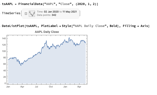
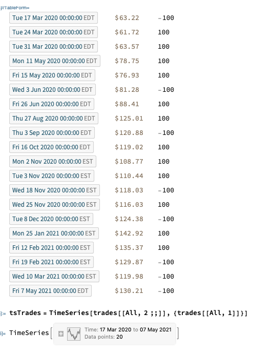
Next, we’ll generate a series of random trades using the AAPL time series, as follows (we also take the opportunity to convert the list of trades into a time series, tsTrades):

trades = Transpose@ Join[Transpose[ tsAAPL["DatePath"][[ Sort@RandomSample[Range[tsAAPL["PathLength"]], 20]]]], {RandomChoice[{-100, 100}, 20]}]; trades // TableForm

Trade P&L Calculation

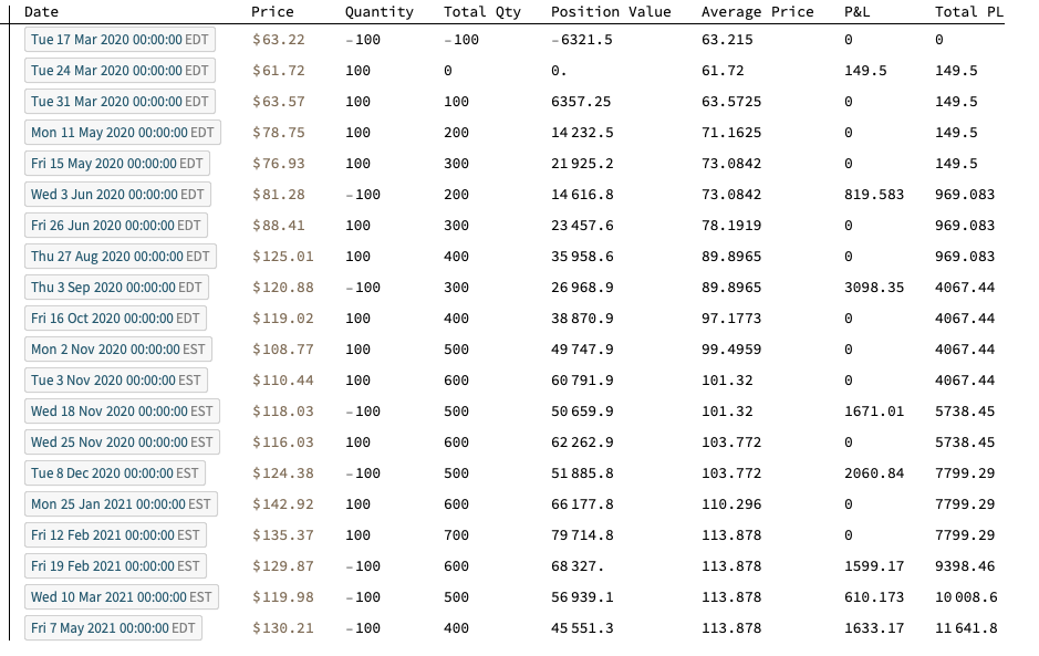
We are now ready to apply our Trade P&L calculation function, first to the list of trades in array form:

TableForm[
Flatten[#] & /@ 
Partition[
Riffle[trades, 
CalculateRealizedPLFromTrades[trades[[All, 2 ;; 3]]]], 2], 
TableHeadings -> {{}, {"Date", "Price", "Quantity", "Total Qty", 
"Position Value", "Average Price", "P&L", "Total PL"}}]

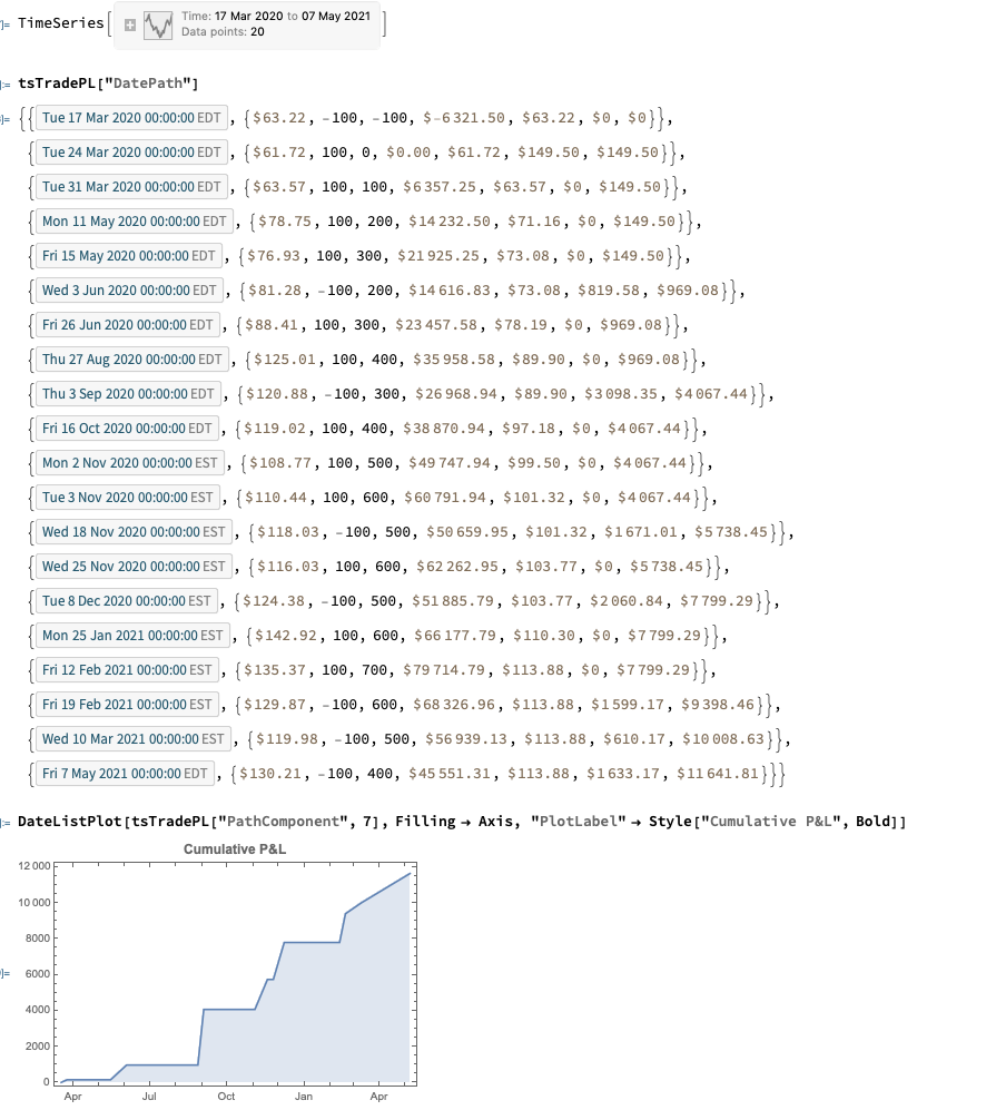
The timeseries version of the function provides the output as a timeseries object in Quantity[“US Dollars”] format and, of course, can be plotted immediately with DateListPlot (it is also convenient for other reasons, as the complete backtest system is built around timeseries objects):

tsTradePL = CalculateRealizedPLFromTrades[tsTrades]

September 29, 2020

Robustness in Quantitative Research and Trading

What is Strategy Robustness? What is its relevance to Quantitative Research and Trading?

One of the most highly desired properties of any financial model or investment strategy, by investors and managers alike, is robustness. I would define robustness as the ability of the strategy to deliver a consistent results across a wide range of market conditions. It, of course, by no means the only desirable property – investing in Treasury bills is also a pretty robust strategy, although the returns are unlikely to set an investor’s pulse racing – but it does ensure that the investor, or manager, is unlikely to be on the receiving end of an ugly surprise when market conditions adjust.

Robustness is not the same thing as low volatility, which also tends to be a characteristic highly prized by many investors. A strategy may operate consistently, with low volatility in certain market conditions, but behave very differently in other. For instance, a delta-hedged short-volatility book containing exotic derivative positions. The point is that empirical researchers do not know the true data-generating process for the markets they are modeling. When specifying an empirical model they need to make arbitrary assumptions. An example is the common assumption that assets returns follow a Gaussian distribution. In fact, the empirical distribution of the great majority of asset process exhibit the characteristic of “fat tails”, which can result from the interplay between multiple market states with random transitions. See this post for details:

http://jonathankinlay.com/2014/05/a-quantitative-analysis-of-stationarity-and-fat-tails/

In statistical arbitrage, for example, quantitative researchers often make use of cointegration models to build pairs trading strategies. However the testing procedures used in current practice are not sufficient powerful to distinguish between cointegrated processes and those whose evolution just happens to correlate temporarily, resulting in the frequent breakdown in cointegrating relationships. For instance, see this post:

http://jonathankinlay.com/2017/06/statistical-arbitrage-breaks/

Modeling Assumptions are Often Wrong – and We Know It

We are, of course, not the first to suggest that empirical models are misspecified:

“All models are wrong, but some are useful” (Box 1976, Box and Draper 1987).

Martin Feldstein (1982: 829): “In practice all econometric specifications are necessarily false models.”

Luke Keele (2008: 1): “Statistical models are always simplifications, and even the most complicated model will be a pale imitation of reality.”

Peter Kennedy (2008: 71): “It is now generally acknowledged that econometric models are false and there is no hope, or pretense, that through them truth will be found.”

During the crash of 2008 quantitative Analysts and risk managers found out the hard way that the assumptions underpinning the copula models used to price and hedge credit derivative products were highly sensitive to market conditions. In other words, they were not robust. See this post for more on the application of copula theory in risk management:

http://jonathankinlay.com/2017/01/copulas-risk-management/

Robustness Testing in Quantitative Research and Trading

We interpret model misspecification as model uncertainty. Robustness tests analyze model uncertainty by comparing a baseline model to plausible alternative model specifications. Rather than trying to specify models correctly (an impossible task given causal complexity), researchers should test whether the results obtained by their baseline model, which is their best attempt of optimizing the specification of their empirical model, hold when they systematically replace the baseline model specification with plausible alternatives. This is the practice of robustness testing.

Robustness testing analyzes the uncertainty of models and tests whether estimated effects of interest are sensitive to changes in model specifications. The uncertainty about the baseline model’s estimated effect size shrinks if the robustness test model finds the same or similar point estimate with smaller standard errors, though with multiple robustness tests the uncertainty likely increases. The uncertainty about the baseline model’s estimated effect size increases of the robustness test model obtains different point estimates and/or gets larger standard errors. Either way, robustness tests can increase the validity of inferences.

Robustness testing replaces the scientific crowd by a systematic evaluation of model alternatives.

Robustness in Quantitative Research

In the literature, robustness has been defined in different ways:

as same sign and significance (Leamer)
as weighted average effect (Bayesian and Frequentist Model Averaging)
as effect stability We define robustness as effect stability.

Parameter Stability and Properties of Robustness

Robustness is the share of the probability density distribution of the baseline model that falls within the 95-percent confidence interval of the baseline model. In formulaeic terms:

Robustness is left-–right symmetric: identical positive and negative deviations of the robustness test compared to the baseline model give the same degree of robustness.
If the standard error of the robustness test is smaller than the one from the baseline model, ρ converges to 1 as long as the difference in point estimates is negligible.
For any given standard error of the robustness test, ρ is always and unambiguously smaller the larger the difference in point estimates.
Differences in point estimates have a strong influence on ρ if the standard error of the robustness test is small but a small influence if the standard errors are large.

Robustness Testing in Four Steps

Define the subjectively optimal specification for the data-generating process at hand. Call this model the baseline model.
Identify assumptions made in the specification of the baseline model which are potentially arbitrary and that could be replaced with alternative plausible assumptions.
Develop models that change one of the baseline model’s assumptions at a time. These alternatives are called robustness test models.
Compare the estimated effects of each robustness test model to the baseline model and compute the estimated degree of robustness.

Model Variation Tests

Model variation tests change one or sometimes more model specification assumptions and replace with an alternative assumption, such as:

change in set of regressors
change in functional form
change in operationalization
change in sample (adding or subtracting cases)

Example: Functional Form Test

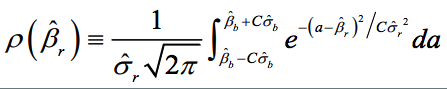
The functional form test examines the baseline model’s functional form assumption against a higher-order polynomial model. The two models should be nested to allow identical functional forms. As an example, we analyze the ‘environmental Kuznets curve’ prediction, which suggests the existence of an inverse u-shaped relation between per capita income and emissions.

Note: grey-shaded area represents confidence interval of baseline model

Another example of functional form testing is given in this review of Yield Curve Models:

http://jonathankinlay.com/2018/08/modeling-the-yield-curve/

Random Permutation Tests

Random permutation tests change specification assumptions repeatedly. Usually, researchers specify a model space and randomly and repeatedly select model from this model space. Examples:

sensitivity tests (Leamer 1978)
artificial measurement error (Plümper and Neumayer 2009)
sample split – attribute aggregation (Traunmüller and Plümper 2017)
multiple imputation (King et al. 2001)

We use Monte Carlo simulation to test the sensitivity of the performance of our Quantitative Equity strategy to changes in the price generation process and also in model parameters:

http://jonathankinlay.com/2017/04/new-longshort-equity/

Structured Permutation Tests

Structured permutation tests change a model assumption within a model space in a systematic way. Changes in the assumption are based on a rule, rather than random. Possibilities here include:

sensitivity tests (Levine and Renelt)
jackknife test
partial demeaning test

Example: Jackknife Robustness Test

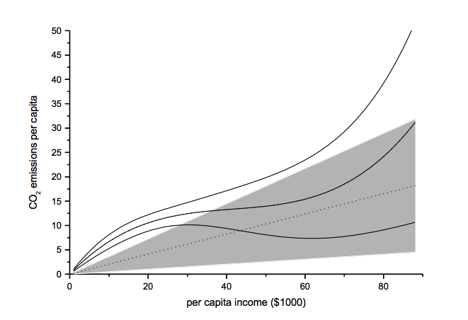
The jackknife robustness test is a structured permutation test that systematically excludes one or more observations from the estimation at a time until all observations have been excluded once. With a ‘group-wise jackknife’ robustness test, researchers systematically drop a set of cases that group together by satisfying a certain criterion – for example, countries within a certain per capita income range or all countries on a certain continent. In the example, we analyse the effect of earthquake propensity on quake mortality for countries with democratic governments, excluding one country at a time. We display the results using per capita income as information on the x-axes.

Upper and lower bound mark the confidence interval of the baseline model.

Robustness Limit Tests

Robustness limit tests provide a way of analyzing structured permutation tests. These tests ask how much a model specification has to change to render the effect of interest non-robust. Some examples of robustness limit testing approaches:

unobserved omitted variables (Rosenbaum 1991)
measurement error
under- and overrepresentation
omitted variable correlation

For an example of limit testing, see this post on a review of the Lognormal Mixture Model:

http://jonathankinlay.com/2018/08/the-lognormal-mixture-variance-model/

Summary on Robustness Testing

Robustness tests have become an integral part of research methodology. Robustness tests allow to study the influence of arbitrary specification assumptions on estimates. They can identify uncertainties that otherwise slip the attention of empirical researchers. Robustness tests offer the currently most promising answer to model uncertainty.

September 24, 2019September 24, 2019

Applications of Graph Theory In Finance

Analyzing Big Data

Very large datasets – comprising voluminous numbers of symbols – present challenges for the analyst, not least of which is the difficulty of visualizing relationships between the individual component assets. Absent the visual clues that are often highlighted by graphical images, it is easy for the analyst to overlook important changes in relationships. One means of tackling the problem is with the use of graph theory.

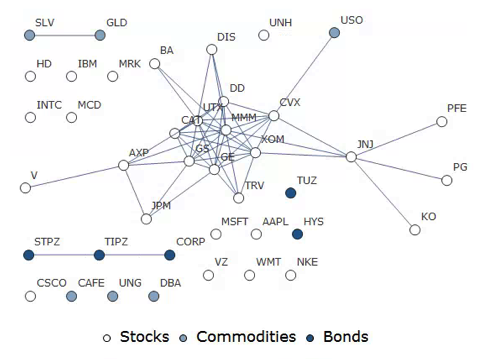
DOW 30 Index Member Stocks Correlation Graph

In this example I have selected a universe of the Dow 30 stocks, together with a sample of commodities and bonds and compiled a database of daily returns over the period from Jan 2012 to Dec 2013. If we want to look at how the assets are correlated, one way is to created an adjacency graph that maps the interrelations between assets that are correlated at some specified level (0.5 of higher, in this illustration).

Obviously the choice of correlation threshold is somewhat arbitrary, and it is easy to evaluate the results dynamically, across a wide range of different threshold parameters, say in the range from 0.3 to 0.75:

The choice of parameter (and time frame) may be dependent on the purpose of the analysis: to construct a portfolio we might select a lower threshold value; but if the purpose is to identify pairs for possible statistical arbitrage strategies, one will typically be looking for much higher levels of correlation.

Correlated Cliques

Reverting to the original graph, there is a core group of highly inter-correlated stocks that we can easily identify more clearly using the Mathematica function FindClique to specify graph nodes that have multiple connections:

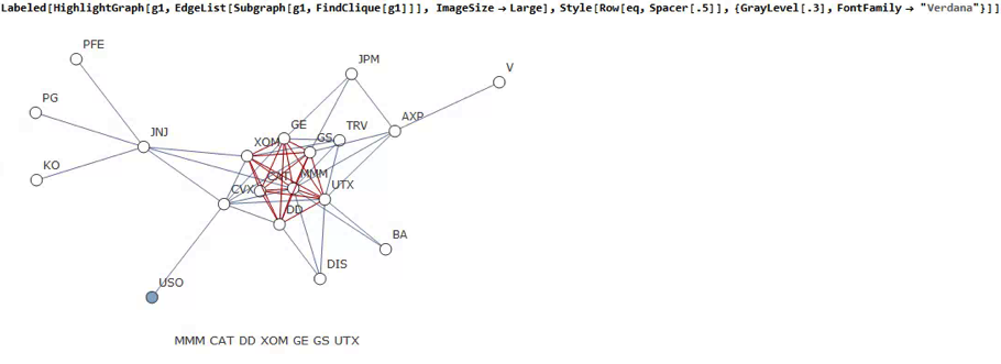
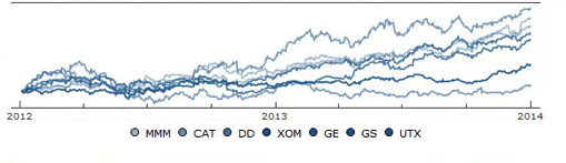
We might, for example, explore the relative performance of members of this sub-group over time and perhaps investigate the question as to whether relative out-performance or under-performance is likely to persist, or, given the correlation characteristics of this group, reverse over time to give a mean-reversion effect.

Constructing a Replicating Portfolio

An obvious application might be to construct a replicating portfolio comprising this equally-weighted sub-group of stocks, and explore how well it tracks the Dow index over time (here I am using the DIA ETF as a proxy for the index, for the sake of convenience):

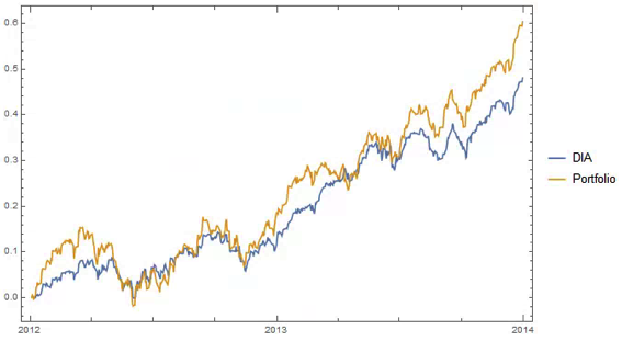
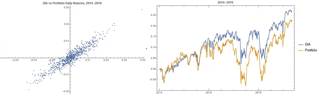
The correlation between the Dow index (DIA ETF) and the portfolio remains strong (around 0.91) throughout the out-of-sample period from 2014-2016, although the performance of the portfolio is distinctly weaker than that of the index ETF after the early part of 2014:

Constructing Robust Portfolios

Another application might be to construct robust portfolios of lower-correlated assets. Here for example we use the graph to identify independent vertices that have very few correlated relationships (designated using the star symbol in the graph below). We can then create an equally weighted portfolio comprising the assets with the lowest correlations and compare its performance against that of the Dow Index.

The new portfolio underperforms the index during 2014, but with lower volatility and average drawdown.

Conclusion – Graph Theory has Applications in Portfolio Constructions and Index Replication

Graph theory clearly has a great many potential applications in finance. It is especially useful as a means of providing a graphical summary of data sets involving a large number of complex interrelationships, which is at the heart of portfolio theory and index replication. Another useful application would be to identify and evaluate correlation and cointegration relationships between pairs or small portfolios of stocks, as they evolve over time, in the context of statistical arbitrage.

October 2, 2018October 2, 2018

Quant Strategies in 2018

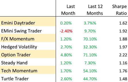
Quant Strategies – Performance Summary Sept. 2018

The end of Q3 seems like an appropriate time for an across-the-piste review of how systematic strategies are performing in 2018. I’m using the dozen or more strategies running on the Systematic Algotrading Platform as the basis for the performance review, although results will obviously vary according to the specifics of the strategy. All of the strategies are traded live and performance results are net of subscription fees, as well as slippage and brokerage commissions.

Volatility Strategies

Those waiting for the hammer to fall on option premium collecting strategies will have been disappointed with the way things have turned out so far in 2018. Yes, February saw a long-awaited and rather spectacular explosion in volatility which completely destroyed several major volatility funds, including the VelocityShares Daily Inverse VIX Short-Term ETN (XIV) as well as Chicago-based hedged fund LJM Partners (“our goal is to preserve as much capital as possible”), that got caught on the wrong side of the popular VIX carry trade. But the lack of follow-through has given many volatility strategies time to recover. Indeed, some are positively thriving now that elevated levels in the VIX have finally lifted option premiums from the bargain basement levels they were languishing at prior to February’s carnage. The Option Trader strategy is a stand-out in this regard: not only did the strategy produce exceptional returns during the February melt-down (+27.1%), the strategy has continued to outperform as the year has progressed and YTD returns now total a little over 69%. Nor is the strategy itself exceptionally volatility: the Sharpe ratio has remained consistently above 2 over several years.

Hedged Volatility Trading

Investors’ chief concern with strategies that rely on collecting option premiums is that eventually they may blow up. For those looking for a more nuanced approach to managing tail risk the Hedged Volatility strategy may be the way to go. Like many strategies in the volatility space the strategy looks to generate alpha by trading VIX ETF products; but unlike the great majority of competitor offerings, this strategy also uses ETF options to hedge tail risk exposure. While hedging costs certainly acts as a performance drag, the results over the last few years have been compelling: a CAGR of 52% with a Sharpe Ratio close to 2.

F/X Strategies

One of the common concerns for investors is how to diversify their investment portfolios, especially since the great majority of assets (and strategies) tend to exhibit significant positive correlation to equity indices these days. One of the characteristics we most appreciate about F/X strategies in general and the F/X Momentum strategy in particular is that its correlation to the equity markets over the last several years has been negligible. Other attractive features of the strategy include the exceptionally high win rate – over 90% – and the profit factor of 5.4, which makes life very comfortable for investors. After a moderate performance in 2017, the strategy has rebounded this year and is up 56% YTD, with a CAGR of 64.5% and Sharpe Ratio of 1.89.

Equity Long/Short

Thanks to the Fed’s accommodative stance, equity markets have been generally benign over the last decade to the benefit of most equity long-only and long-short strategies, including our equity long/short Turtle Trader strategy , which is up 31% YTD. This follows a spectacular 2017 (+66%) , and is in line with the 5-year CAGR of 39%. Notably, the correlation with the benchmark S&P500 Index is relatively low (0.16), while the Sharpe Ratio is a respectable 1.47.

Equity ETFs – Market Timing/Swing Trading

One alternative to the traditional equity long/short products is the Tech Momentum strategy. This is a swing trading strategy that exploits short term momentum signals to trade the ProShares UltraPro QQQ (TQQQ) and ProShares UltraPro Short QQQ (SQQQ) leveraged ETFs. The strategy is enjoying a banner year, up 57% YTD, with a four-year CAGR of 47.7% and Sharpe Ratio of 1.77. A standout feature of this equity strategy is its almost zero correlation with the S&P 500 Index. It is worth noting that this strategy also performed very well during the market decline in Feb, recording a gain of over 11% for the month.

Futures Strategies

It’s a little early to assess the performance of the various futures strategies in the Systematic Strategies portfolio, which were launched on the platform only a few months ago (despite being traded live for far longer). For what it is worth, both of the S&P 500 E-Mini strategies, the Daytrader and the Swing Trader, are now firmly in positive territory for 2018. Obviously we are keeping a watchful eye to see if the performance going forward remains in line with past results, but our experience of trading these strategies gives us cause for optimism.

Conclusion: Quant Strategies in 2018

There appear to be ample opportunities for investors in the quant sector across a wide range of asset classes. For investors with equity market exposure, we particularly like strategies with low market correlation that offer significant diversification benefits, such as the F/X Momentum and F/X Momentum strategies. For those investors seeking the highest risk adjusted return, option selling strategies like the Option Trader strategy are the best choice, while for more cautious investors concerned about tail risk the Hedged Volatility strategy offers the security of downside protection. Finally, there are several new strategies in equities and futures coming down the pike, several of which are already showing considerable promise. We will review the performance of these newer strategies at the end of the year.

Go here for more information about the Systematic Algotrading Platform.