Just in Time: Programming Grows Up – JonathanKinlay.com

Move over C++: Modern Programming Languages Combine Productivity and Efficiency

Like many in the field of quantitative research, I have programmed in several different languages over the years: Assembler, Fortran, Algol, Pascal, APL, VB, C, C++, C#, Matlab, R, Mathematica.  There is an even longer list of languages I have never bothered with:  Cobol, Java, Python, to name but three.

In general, the differences between many of these are much fewer than their similarities:  they reserve memory; they have operators; they loop.  Several have ghastly syntax requiring random punctuation that supposedly makes the code more intelligible, but in practice does precisely the opposite.  Some, like Objective C, are so ugly and poorly designed they should have been strangled at birth.  The ubiquity of C is due, not to its elegance, but to the fact that it was one of the first languages distributed for free to impecunious students.  The greatest benefit of most languages is that they compile to machine code that executes quickly.  But the task of coding in them is often an unpleasant, inefficient process that typically involves reinvention of the wheel multiple times over and massive amounts of tedious debugging.   Who, after all, doesn’t enjoy unintelligible error messages like “parsec error in dynamic memory heap allocator” – when the alternative, comprehensible version would be so prosaic:  “in line 51 you missed one of those curly brackets we insist on for no good reason”.

There have been relatively few steps forward that actually have had any real significance.  Most times, the software industry operates rather like the motor industry:  while the consumer pines for, say, a new kind of motor that will do 1,000 miles to the gallon without looking like an electric golf cart, manufacturers announce, to enormous fanfare, trivia like heated wing mirrors.

SSALGOTRADING AD

The first language I came across that seemed like a material advance was APL, a matrix-based language that offers lots of built-in functionality, very much like MatLab.  Achieving useful end-results in a matter of days or weeks, rather than months, remains one of the great benefits of such high-level languages. Unfortunately, like all high-level languages that are weakly typed, APL, MatLab, R, etc, are interpreted rather than compiled. And so I learned about the perennial trade-off that has plagued systems development over the last 30 years: programming productivity vs. execution efficiency.  The great divide between high level, interpreted languages and lower-level, compiled languages, would remain forever, programming language experts assured us, because of the lack of type-specificity in the former.

High-level language designers did what they could, offering ever-larger collections of sophisticated, built-in operators and libraries that use efficient machine-code instructions, as well as features such as parallel processing, to speed up execution.  But, while it is now feasible to develop smaller applications in a few lines of  Matlab or Mathematica that have perfectly acceptable performance characteristics, major applications (trading platforms, for example) seemed ordained to languish forever in the province of languages whose chief characteristic appears to be the lack of intelligibility of their syntax.

I was always suspicious of this thesis.  It seemed to me that it should not be beyond the wit of man to design a programming language that offers straightforward, type-agnostic syntax that can be compiled.  And lo:  this now appears to have come true.

Of the multitude of examples that will no doubt be offered up over the next several years I want to mention two – not because I believe them to be the “final word” on this important topic, but simply as exemplars of what is now possible, as well as harbingers of what is to come.

Trading Technologies ADL 

ADL

The first, Trading Technologies’ ADL, I have written about at length already.  In essence, ADL is a visual programming language focused on trading system development.  ADL allows the programmer to deploy highly-efficient, pre-built code blocks as icons that are dragged and dropped onto a programming canvass and assembled together using logic connections represented by lines drawn on the canvass.  From my experience, ADL outpaces any other high-level development tool by at least an order of magnitude, but without sacrificing (much) efficiency in execution, firstly because the code blocks are written in native C#, and secondly, because completed systems are deployed on an algo server with a sub-millisecond connectivity to the exchange.


Julia

The second example is a language called Julia, which you can find out more about here.  To quote from the web site:

“Julia is a high-level, high-performance dynamic programming language for technical computing.  Julia features optional typing, multiple dispatch, and good performance, achieved using type inference and just-in-time (JIT) compilation, implemented using LLVM

The language syntax is indeed very straightforward and logical.  As to performance, the evidence appears to be that it is possible to achieve execution speeds that match or even exceed those achieved by languages like Java or C++.

How High Level Programming Languages Match Up

The following micro-benchmark results, provided on the Julia web site, were obtained on a single core (serial execution) on an Intel® Xeon® CPU E7-8850 2.00GHz CPU with 1TB of 1067MHz DDR3 RAM, running Linux:

Benchmark

We need not pretend that this represents any kind of comprehensive speed test of Julia or its competitors.  Still, it’s worth dwelling on a few of the salient results.  The first thing that strikes me is how efficient Fortran, the grand-daddy of programming languages, remains in comparison to more modern alternatives, including the C benchmark.   The second result I find striking is how slow the much-touted Python is compared to Julia, Go and C.  The third result is how poorly MatLab, Octave and R perform on several of the tests.  Finally, and in some ways the greatest surprise at all is the execution efficiency of Mathematica relative to other high-level languages like MatLab and R.  It appears that Wolfram has made enormous progress in improving the speed of Mathematica, presumably through the vast expansion of highly efficient built-in operators and functions that have been added in recent releases (see chart below).

mathematica fns

Source:  Wolfram

Mathematica even compares favorably to Python on several of the tests.  Given that, why would anyone spend time learning a language like Python, which offers neither the development advantages of Mathematica, nor the speed advantages of C (or Fortran, Java or Julia)?

In any event, the main point is this:  it appears that, in 2015, we can finally look forward to dispensing with legacy programing languages and their primitive syntax and instead develop large, scalable systems that combine programming productivity and execution efficiency.  And that is reason enough for any self-respecting quant to rejoice.

My best wishes to you all for the New Year.

Money Management – the Good, the Bad and the Ugly

The infatuation of futures traders with the subject of money management, (more aptly described as position sizing), is something of a puzzle for someone coming from a background in equities or forex.  The idea is, simply, that one can improve one’s  trading performance through the judicious use of leverage, increasing the size of a position at times and reducing it at others.

MM Grapgic

Perhaps the most widely known money management technique is the Martingale, where the size of the trade is doubled after every loss.  It is easy to show mathematically that such a system must win eventually, provided that the bet size is unlimited.  It is also easy to show that, small as it may be, there is a non-zero probability of a long string of losing trades that would bankrupt the trader before he was able to recoup all his losses.  Still, the prospect offered by the Martingale strategy is an alluring one: the idea that, no matter what the underlying trading strategy, one can eventually be certain of winning.  And so a virtual cottage industry of money management techniques has evolved.

One of the reasons why the money management concept is prevalent in the futures industry compared to, say, equities or f/x, is simply the trading mechanics.  Doubling the size of a position in futures might mean trading an extra contract, or perhaps a ten-lot; doing the same in equities might mean scaling into and out of multiple positions comprising many thousands of shares.  The execution risk and cost of trying to implement a money management program in equities has historically made the  idea infeasible, although that is less true today, given the decline in commission rates and the arrival of smart execution algorithms.  Still, money management is a concept that originated in the futures industry and will forever be associated with it.

SSALGOTRADING AD

Van Tharp on Position Sizing
I was recently recommended to read Van Tharp’s Definitive Guide to Position Sizing, which devotes several hundred pages to the subject.  Leaving aside the great number of pages of simulation results, there is much to commend it.  Van Tharp does a pretty good job of demolishing highly speculative and very dangerous “money management” techniques such as the Kelly Criterion and Ralph Vince’s Optimal f, which make unrealistic assumptions of one kind or another, such as, for example, that there are only two outcomes, rather than the multiple possibilities from a trading strategy, or considering only the outcome of a single trade, rather than a succession of trades (whose outcome may not be independent).  Just as  with the Martingale, these techniques will often produce unacceptably large drawdowns.  In fact, as I have pointed out elsewhere, the use of leverage which many so-called money management techniques actually calls for increases in the risk in the original strategy, often reducing its risk-adjusted return.

As Van Tharp points out, mathematical literacy is not one of the strongest suits of futures traders in general and the money management strategy industry reflects that.

But Van Tharp  himself is not immune to misunderstanding mathematical concepts.  His central idea is that trading systems should be rated according to its System Quality Number, which he defines as:

SQN  = (Expectancy / standard deviation of R) * square root of Number of Trades

R is a central concept of Van Tharp’s methodology, which he defines as how much you will lose per unit of your investment.  So, for example, if you buy a stock today for $50 and plan to sell it if it reaches $40,  your R is $10.  In cases like this you have a clear definition of your R.  But what if you don’t?  Van Tharp sensibly recommends you use your average loss as an estimate of R.

Expectancy, as Van Tharp defines it, is just the expected profit per trade of the system expressed as a multiple of R.  So

SQN = ( (Average Profit per Trade / R) / standard deviation (Average Profit per Trade / R) * square root of Number of Trades

Squaring both sides of the equation, we get:

SQN^2  =  ( (Average Profit per Trade )^2 / R^2) / Variance (Average Profit per Trade / R) ) * Number of Trades

The R-squared terms cancel out, leaving the following:

SQN^2     =  ((Average Profit per Trade ) ^ 2 / Variance (Average Profit per Trade)) *  Number of Trades

Hence,

SQN = (Average Profit per Trade / Standard Deviation (Average Profit per Trade)) * square root of Number of Trades

There is another name by which this measure is more widely known in the investment community:  the Sharpe Ratio.

On the “Optimal” Position Sizing Strategy
In my view,  Van Tharp’s singular achievement has been to spawn a cottage industry out of restating a fact already widely known amongst investment professionals, i.e. that one should seek out strategies that maximize the Sharpe Ratio.

Not that seeking to maximize the Sharpe Ratio is a bad idea – far from it.  But then Van Tharp goes on to suggest that one should consider only strategies with a SQN of greater than 2, ideally much higher (he mentions SQNs of the order of 3-6).

But 95% or more of investable strategies have a Sharpe Ratio less than 2.  In fact, in the world of investment management a Sharpe Ratio of 1.5 is considered very good.  Barely a handful of funds have demonstrated an ability to maintain a Sharpe Ratio of greater than 2 over a sustained period (Jim Simon’s Renaissance Technologies being one of them).  Only in the world of high frequency trading do strategies typically attain the kind of Sharpe Ratio (or SQN) that Van Tharp advocates.  So while Van Tharp’s intentions are well meaning, his prescription is unrealistic, for the majority of investors.

One recommendation of Van Tharp’s that should be taken seriously is that there is no single “best” money management strategy that suits every investor.  Instead, position sizing should be evolved through simulation, taking into account each trader or investor’s preferences in terms of risk and return.  This makes complete sense: a trader looking to make 100% a year and willing to risk 50% of his capital is going to adopt a very different approach to money management, compared to an investor who will be satisfied with a 10% return, provided his risk of losing money is very low.  Again, however, there is nothing new here:  the problem of optimal allocation based on an investor’s aversion to risk has been thoroughly addressed in the literature for at least the last 50 years.

What about the Equity Curve Money Management strategy I discussed in a previous post?  Isn’t that a kind of Martingale?  Yes and no.  Indeed, the strategy does require us to increase the original investment after a period of loss. But it does so, not after a single losing trade, but after a series of losses from which the strategy is showing evidence of recovering.  Furthermore, the ECMM system caps the add-on investment at some specified level, rather than continuing to double the trade size after every loss, as in a Martingale.

But the critical difference between the ECMM and the standard Martingale lies in the assumptions about dependency in the returns of the underlying strategy. In the traditional Martingale, profits and losses are independent from one trade to the next.  By contrast, scenarios where ECMM is likely to prove effective are ones where there is dependency in the underlying strategy, more specifically, negative autocorrelation in returns over some horizon.  What that means is that periods of losses or lower returns tend to be followed by periods of gains, or higher returns.  In other words, ECMM works when the underlying strategy has a tendency towards mean reversion.

CONCLUSION
The futures industry has spawned a myriad of position sizing strategies.  Many are impractical, or positively dangerous, leading as they do to significant risk of catastrophic loss.  Generally, investors should seek out strategies with higher Sharpe Ratios, and use money management techniques only to improve the risk-adjusted return.  But there is no universal money management methodology that will suit every investor.  Instead, money management should be conditioned on each individual investors risk preferences.

Building Systematic Strategies – A New Approach

Anyone active in the quantitative space will tell you that it has become a great deal more competitive in recent years.  Many quantitative trades and strategies are a lot more crowded than they used to be and returns from existing  strategies are on the decline.

THE CHALLENGE

The Challenge

Meanwhile, costs have been steadily rising, as the technology arms race has accelerated, with more money being spent on hardware, communications and software than ever before.  As lead times to develop new strategies have risen, the cost of acquiring and maintaining expensive development resources have spiraled upwards.  It is getting harder to find new, profitable strategies, due in part to the over-grazing of existing methodologies and data sets (like the E-Mini futures, for example). There has, too, been a change in the direction of quantitative research in recent years.  Where once it was simply a matter of acquiring the fastest pipe to as many relevant locations as possible, the marginal benefit of each extra $ spent on infrastructure has since fallen rapidly.  New strategy research and development is now more model-driven than technology driven.


THE OPPORTUNITY

The Opportunity

What is needed at this point is a new approach:  one that accelerates the process of identifying new alpha signals, prototyping and testing new strategies and bringing them into production, leveraging existing battle-tested technologies and trading platforms.


GENETIC PROGRAMMING

Genetic programming, which has been around since the 1990’s when its use was pioneered in proteomics, enjoys significant advantages over traditional research and development methodologies.

GP

GP is an evolutionary-based algorithmic methodology in which a system is given a set of simple rules, some data, and a fitness function that produces desired outcomes from combining the rules and applying them to the data.   The idea is that, by testing large numbers of possible combinations of rules, typically in the  millions, and allowing the most successful rules to propagate, eventually we will arrive at a strategy solution that offers the required characteristics.

ADVANTAGES OF GENETIC PROGRAMMING

AdvantagesThe potential benefits of the GP approach are considerable:  not only are strategies developed much more quickly and cost effectively (the price of some software and a single CPU vs. a small army of developers), the process is much more flexible. The inflexibility of the traditional approach to R&D is one of its principle shortcomings.  The researcher produces a piece of research that is subsequently passed on to the development team.  Developers are usually extremely rigid in their approach: when asked to deliver X, they will deliver X, not some variation on X.  Unfortunately research is not an exact science: what looks good in a back-test environment may not pass muster when implemented in live trading.  So researchers need to “iterate around” the idea, trying different combinations of entry and exit logic, for example, until they find a variant that works.  Developers are lousy at this;  GP systems excel at it.

CHALLENGES FOR THE GENETIC PROGRAMMING APPROACH

So enticing are the potential benefits of GP that it begs the question as to why the approach hasn’t been adopted more widely.  One reason is the strong preference amongst researchers for an understandable – and testable – investment thesis.  Researchers – and, more importantly, investors –  are much more comfortable if they can articulate the premise behind a strategy.  Even if a trade turns out to be a loser, we are generally more comfortable buying a stock on the supposition of, say,  a positive outcome of a pending drug trial, than we are if required to trust the judgment of a black box, whose criteria are inherently unobservable.

GP Challenges

Added to this, the GP approach suffers from three key drawbacks:  data sufficiency, data mining and over-fitting.  These are so well known that they hardly require further rehearsal.  There have been many adverse outcomes resulting from poorly designed mechanical systems curve fitted to the data. Anyone who was active in the space in the 1990s will recall the hype over neural networks and the over-exaggerated claims made for their efficacy in trading system design.  Genetic Programming, a far more general and powerful concept,  suffered unfairly from the ensuing adverse publicity, although it does face many of the same challenges.

A NEW APPROACH

I began working in the field of genetic programming in the 1990’s, with my former colleague Haftan Eckholdt, at that time head of neuroscience at Yeshiva University, and we founded a hedge fund, Proteom Capital, based on that approach (large due to Haftan’s research).  I and my colleagues at Systematic Strategies have continued to work on GP related ideas over the last twenty years, and during that period we have developed a methodology that address the weaknesses that have held back genetic programming from widespread adoption.

Advances

Firstly, we have evolved methods for transforming original data series that enables us to avoid over-using the same old data-sets and, more importantly, allows new patterns to be revealed in the underlying market structure.   This effectively eliminates the data mining bias that has plagued the GP approach. At the same time, because our process produces a stronger signal relative to the background noise, we consume far less data – typically no more than a couple of years worth.

Secondly, we have found we can enhance the robustness of prototype strategies by using double-blind testing: i.e. data sets on which the performance of the model remains unknown to the machine, or the researcher, prior to the final model selection.

Finally, we are able to test not only the alpha signal, but also multiple variations of the trade expression, including different types of entry and exit logic, as well as profit targets and stop loss constraints.

OUTCOMES:  ROBUST, PROFITABLE STRATEGIES

outcomes

Taken together, these measures enable our GP system to produce strategies that not only have very high performance characteristics, but are also extremely robust.  So, for example, having constructed a model using data only from the continuing bull market in equities in 2012 and 2013, the system is nonetheless capable of producing strategies that perform extremely well when tested out of sample over the highly volatility bear market conditions of 2008/09.

So stable are the results produced by many of the strategies, and so well risk-controlled, that it is possible to deploy leveraged money-managed techniques, such as Vince’s fixed fractional approach.  Money management schemes take advantage of the high level of consistency in performance to increase the capital allocation to the strategy in a way that boosts returns without incurring a high risk of catastrophic loss.  You can judge the benefits of applying these kinds of techniques in some of the strategies we have developed in equity, fixed income, commodity and energy futures which are described below.

CONCLUSION

After 20-30 years of incubation, the Genetic Programming approach to strategy research and development has come of age. It is now entirely feasible to develop trading systems that far outperform the overwhelming majority of strategies produced by human researchers, in a fraction of the time and for a fraction of the cost.

SAMPLE GP SYSTEMS

Sample

SSALGOTRADING AD

emini    emini MM

NG  NG MM

SI MMSI

US US MM


Quantitative Analysis of Fat Tails – JonathanKinlay.com

In this quantitative analysis I explore how, starting from the assumption of a stable, Gaussian distribution in a returns process, we evolve to a system that displays all the characteristics of empirical market data, notably time-dependent moments, high levels of kurtosis and fat tails.  As it turns out, the only additional assumption one needs to make is that the market is periodically disturbed by the random arrival of news.

NOTE:  if you are unable to see the Mathematica models below, you can download the free Wolfram CDF player and you may also need this plug-in.

You can also download the complete Mathematica CDF file here.

Stationarity

A stationary process is one that evolves over time, but whose probability distribution does not vary with time. As the word implies, such a process is stable. More formally, the moments of the distribution are independent of time.

Let’s assume we are dealing with such a process that have constant mean μ and constant volatility (standard deviation) σ.

 Φ=NormalDistribution[μ,σ]

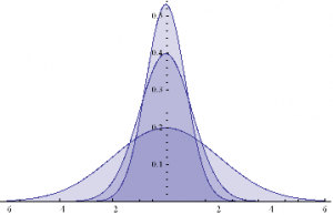
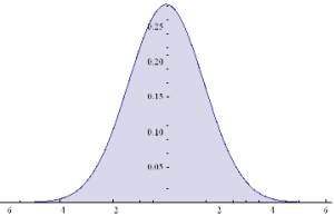
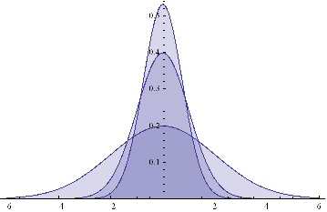
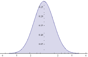
Here are some examples of Normal probability distributions, with constant mean μ = 0 and standard deviation σ ranging from 0.75 to 2

 Plot[Evaluate@Table[PDF[Φ,x],{σ,{.75,1,2}}]/.μ→0,{x,-6,6},Filling→Axis]


Chart 1

The moments of Φ are given by:

 Through[{Mean, StandardDeviation, Skewness, Kurtosis}[Φ]]

{μ,  σ,  0,   3}

They, too, are time – independent.

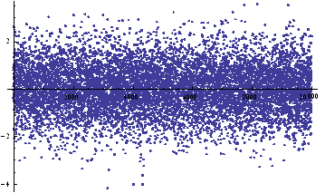
We can simulate some observations from such a process, with, say, mean μ = 0 and standard deviation σ = 1:

ListPlot[sampleData=RandomVariate[Φ /.{μ→0, σ→1},10^4]]


Chart 2

Histogram[sampleData]

Chart 3

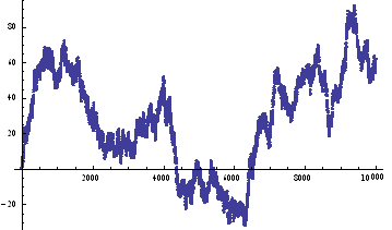
If we assume for the moment that such a process is an adequate description of an asset returns process, we can simulate the evolution of a price process as follows :

ListPlot[prices=Accumulate[sampleData]]

Chart 4


SSALGOTRADING AD

An Empirical Distribution

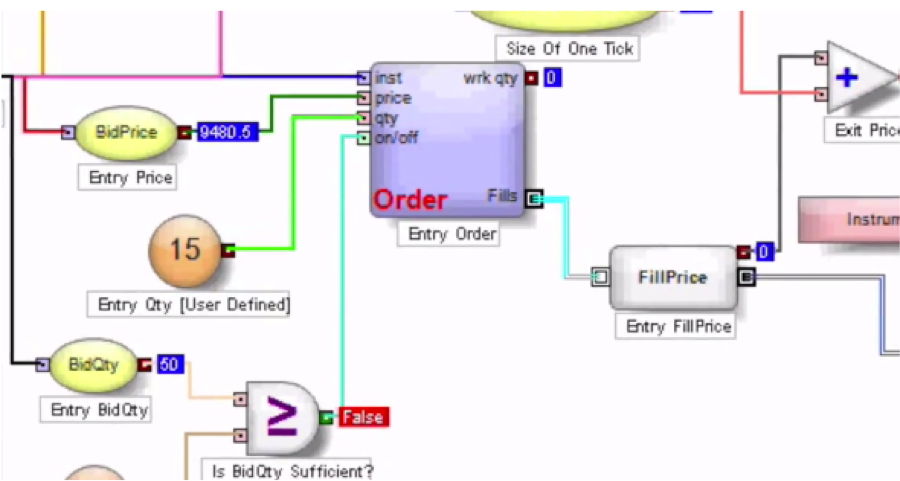
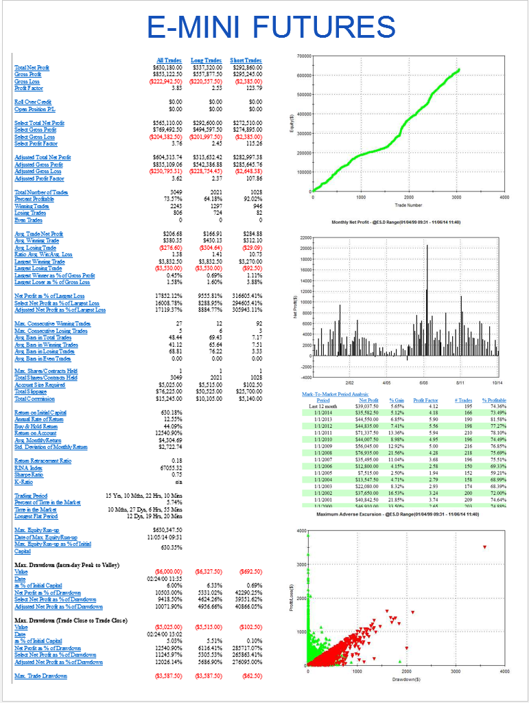
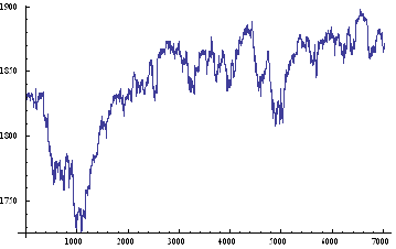
Lets take a look at a real price series, comprising 1 – minute bar data in the June ‘ 14 E – Mini futures contract.

Chart 5

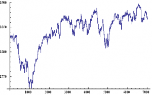
As with our simulated price process, it is clear that the real price process for Emini futures is also non – stationary.

What about the returns process?
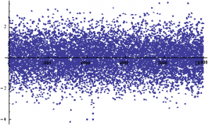
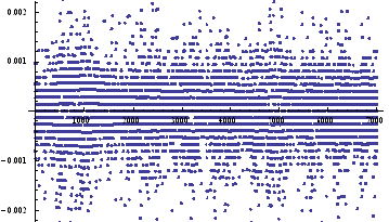
ListPlot[returnsES]

Chart 6

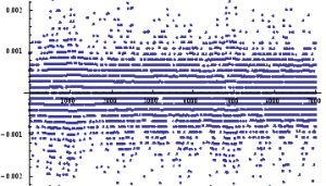
Notice the banding effect in returns, which results from having a fixed, minimum price move of $12 .50, rather than a continuous scale.

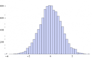
Histogram[returnsES]


Chart 7

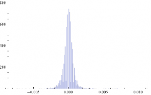
Through[{Min,Max,Mean,Median,StandardDeviation,Skewness,Kurtosis}[returnsES]]

{-0.00867214,  0.0112353,  2.75501×10⁻⁶,   0.,   0.000780895,   0.35467,   26.2376}

The empirical returns distribution doesn’ t appear to be Gaussian – the distribution is much more peaked than a standard Normal distribution with the same mean and standard deviation. And the higher moments don’t fit the Normal model either – the empirical distribution has positive skew and a kurtosis that is almost 9x greater than a Gaussian distribution. The latter signifies what is often referred to as “fat tails”: the distribution has much greater weight in the tails than a standard Normal distribution, indicating a much greater likelihood of an extreme value than a Normal distribution would predict.

A Quantitative Analysis of Non-Stationarity: Two States

Non – stationarity arises when one or more of the moments of a distribution vary over time. Let’s take a look at how that can arise, and its effects.Suppose we have a Gaussian returns process for which the mean, or drift, or trend, fluctuates over time.

Let’s consider a simple example where the process drift is  μ1 and volatility σ1 for most of the time and then for some proportion of time k, we get addition drift  μ2 and volatility σ2.  In other words we have:

 Φ1=NormalDistribution[μ1,σ1]

 Through[{Mean,StandardDeviation,Skewness,Kurtosis}[Φ1]]

{μ1,   σ1,   0,   3}

 Φ2=NormalDistribution[μ2,σ2]

 Through[{Mean,StandardDeviation,Skewness,Kurtosis}[Φ2]]

{μ2,   σ2,   0,   3}

This simple model fits a scenario in which we suppose that the returns process spends most of its time in State 1, in which is Normally distributed with  drift is  μ1 and volatility σ1, and suffers from the occasional “shock” which propels the systems into a second State 2, in which its distribution is a combination of its original distribution and a new Gaussian distribution with different mean and volatility.

Let’ s suppose that we sample the combined process y =  Φ1 + k  Φ2.   What distribution would it have?  We can represent this is follows :

 y=TransformedDistribution[(x1+k x2),{x11,x22}]


Eqn2
 

 Through[{Mean,StandardDeviation,Skewness,Kurtosis}[y]]

Stationarity_52

 Plot[PDF[y,x]/.{μ10,μ20,σ1 1,σ2 2, k0.5},{x,-6,6},FillingAxis]

Chart 8

The result is just another Normal distribution. Depending on the incidence k, y will follow a Gaussian distribution whose mean and variance depend on the mean and variance of the two Normal distributions being mixed. The resulting distribution in State 2 may have higher or lower drift and volatility, but it is still Gaussian, with constant kurtosis of 3.

In other words, the system y will be non-stationary, because the first and second moments change over time, depending on what state it is in. But the form of the distribution is unchanged – it is still Gaussian. There are no fat-tails.

Non – Stationarity : Random States

In the above example the system moved between states in a known, predictable way. The “shocks” to the system were not really shocks, but transitions. But that’s not how financial markets behave: markets move from one state to another in an unpredictable way, with the arrival of news.

We can simulate this situation as follows. Using the former model as a starting point, lets now relax the assumption that the incidence of the second state, k, is a constant. Instead, let’ s assume that k is itself a random variable. In other words we are going to now assume that our system changes state in a random way. How does this alter the distribution?

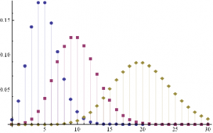
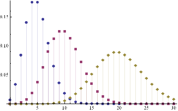
An appropriate model for λ might be a Poisson process, which is often used as a model for unpredictable, discrete events, ranging from bus arrivals to earthquakes.  PDFs of Poisson distributions with means  λ=5, 10 and 20 are shown in the chart below.  These represent probability distributions for processes that have mean  arrivals of 5, 10 or 20 events.

 DiscretePlot[Evaluate@Table[PDF[PoissonDistribution[λ],k],{λ,{5,10,20}}],{k,0,30},PlotRangeAll,PlotMarkersAutomatic]

Chart 9

Our new model now looks like this :

 y=TransformedDistribution[{x1+k*x2},{x1⎡Φ1,x2⎡Φ2,kPoissonDistribution[λ]}]

The first two moments of the distribution are as follows :

Through[{Mean,StandardDeviation}[y]]

Stationarity_60

As before, the mean and standard deviation of the distribution are going to vary, depending on the state of the system, and the mean arrival rate of shocks, . But what about kurtosis? Is it still constant?
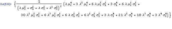
Kurtosis[y]

Eqn1

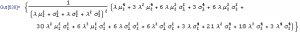
Emphatically not!  The fourth moment of the distribution is now dependent on the drift in the second state, the volatilities of both states and the mean arrival rate of shocks, λ.

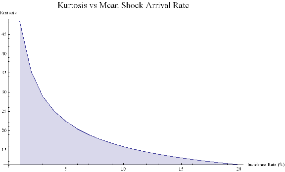
Let’ s look at a specific example.  Assume that in State 1 the process has volatility of 7.5 %, with zero drift, and that the shock distribution also has zero drift with volatility of 65 %. If the mean incidence rate of shocks λ = 10 %, the distribution kurtosis is close to that seen in the empirical distribution for the E-Mini.

 Kurtosis[y] /.{σ10.075,μ20,σ20.65,λ→0.1}

{35.3551}

More generally :

 ListLinePlot[Flatten[Kurtosis[y]/.Table[{σ10.075,μ20,σ20.65,λ→i/20},{i,1,20}]],PlotLabelStyle[“Kurtosis vs Mean Shock Arrival Rate”, FontSize18],AxesLabel->{“Incidence Rate (%)”, “Kurtosis”},FillingAxis, ImageSizeLarge]


Chart 10

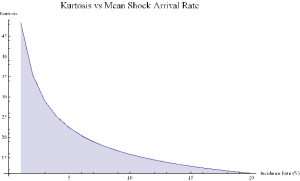
Thus we can see how, even if the underlying returns distribution is Gaussian in form, the random arrival of news “shocks” to the system can induce non – stationarity in overall drift and volatility. It can also result in fat tails. More specifically, if the arrival of news is stochastic in nature, rather than deterministic, the process may exhibit far higher levels of kurtosis than in its original Gaussian state, in which the fourth moment was a constant level of 3.

Quantitative Analysis of a Jump Diffusion Process

Nobel – prize winning economist Robert Merton extended this basic concept to the realm of stochastic calculus.

In Merton’s jump diffusion model, the stock price follows the random process

∂St / St =μdt + σdWt+(J-1)dNt

The first two terms are familiar from the Black–Scholes model : drift rate μ, volatility σ, and random walk Wt (Wiener process).The last term represents the jumps :J is the jump size as a multiple of stock price, while Nt is the number of jump events that have occurred up to time t.is assumed to follow the Poisson process.

 PDF[PoissonDistribution[λt]]

where λ is the average frequency with which jumps occur.

The jump size J follows a log – normal distribution

 PDF[LogNormalDistribution[m, ν], s]

where m is the average jump size and v is the volatility of the jump size.

In the jump diffusion model, the stock price St follows the random process dSt/St=μ dt+σ dWt+(J-1) dN(t), which comprises, in order, drift, diffusive, and jump components. The jumps occur according to a Poisson distribution and their size follows a log-normal distribution. The model is characterized by the diffusive volatility σ, the average jump size J (expressed as a fraction of St), the frequency of jumps λ, and the volatility of jump size ν.

The Volatility Smile

The “implied volatility” corresponding to an option price is the value of the volatility parameter for which the Black-Scholes model gives the same price. A well-known phenomenon in market option prices is the “volatility smile”, in which the implied volatility increases for strike values away from the spot price. The jump diffusion model is a generalization of Black–Scholes in which the stock price has randomly occurring jumps in addition to the random walk behavior. One of the interesting properties of this model is that it displays the volatility smile effect. In this Demonstration, we explore the Black–Scholes implied volatility of option prices (equal for both put and call options) in the jump diffusion model. The implied volatility is modeled as a function of the ratio of option strike price to spot price.