Crash-Proof Investing

As markets continue to make new highs against a backdrop of ever diminishing participation and trading volume, investors have legitimate reasons for being concerned about prospects for the remainder of 2016 and beyond, even without consideration to the myriad of economic and geopolitical risks that now confront the US and global economies. Against that backdrop, remaining fully invested is a test of nerves for those whose instinct is that they may be picking up pennies in front an oncoming steamroller.  On the other hand, there is a sense of frustration in cashing out, only to watch markets surge another several hundred points to new highs.

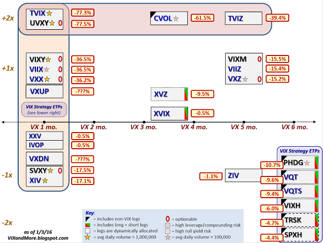
In this article I am going to outline some steps investors can take to match their investment portfolios to suit current market conditions in a way that allows them to remain fully invested, while safeguarding against downside risk.  In what follows I will be using our own Strategic Volatility Strategy, which invests in volatility ETFs such as the iPath S&P 500 VIX ST Futures ETN (NYSEArca:VXX) and the VelocityShares Daily Inverse VIX ST ETN (NYSEArca:XIV), as an illustrative example, although the principles are no less valid for portfolios comprising other ETFs or equities.

SSALGOTRADING AD

Risk and Volatility

Risk may be defined as the uncertainty of outcome and the most common way of assessing it in the context of investment theory is by means of the standard deviation of returns.  One difficulty here is that one may never ascertain the true rate of volatility – the second moment – of a returns process; one can only estimate it.  Hence, while one can be certain what the closing price of a stock was at yesterday’s market close, one cannot say what the volatility of the stock was over the preceding week – it cannot be observed the way that a stock price can, only estimated.  The most common estimator of asset volatility is, of course, the sample standard deviation.  But there are many others that are arguably superior:  Log-Range, Parkinson, Garman-Klass to name but a few (a starting point for those interested in such theoretical matters is a research paper entitled Estimating Historical Volatility, Brandt & Kinlay, 2005).

Leaving questions of estimation to one side, one issue with using standard deviation as a measure of risk is that it treats upside and downside risk equally – the “risk” that you might double your money in an investment is regarded no differently than the risk that you might see your investment capital cut in half.  This is not, of course, how investors tend to look at things: they typically allocate a far higher cost to downside risk, compared to upside risk.

One way to address the issue is by using a measure of risk known as the semi-deviation.  This is estimated in exactly the same way as the standard deviation, except that it is applied only to negative returns.  In other words, it seeks to isolate the downside risk alone.

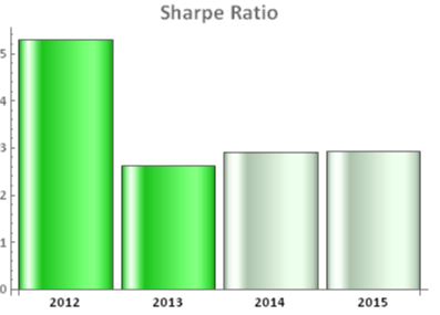
This leads directly to a measure of performance known as the Sortino Ratio.  Like the more traditional Sharpe Ratio, the Sortino Ratio is a measure of risk-adjusted performance – the average return produced by an investment per unit of risk.  But, whereas the Sharpe Ratio uses the standard deviation as the measure of risk, for the Sortino Ratio we use the semi-deviation. In other words, we are measuring the expected return per unit of downside risk.

There may be a great deal of variation in the upside returns of a strategy that would penalize the risk-adjusted returns, as measured by its Sharpe Ratio. But using the Sortino Ratio, we ignore the upside volatility entirely and focus exclusively on the volatility of negative returns (technically, the returns falling below a given threshold, such as the risk-free rate.  Here we are using zero as our benchmark).  This is, arguably, closer to the way most investors tend to think about their investment risk and return preferences.

In a scenario where, as an investor, you are particularly concerned about downside risk, it makes sense to focus on downside risk.  It follows that, rather than aiming to maximize the Sharpe Ratio of your investment portfolio, you might do better to focus on the Sortino Ratio.


Factor Risk and Correlation Risk

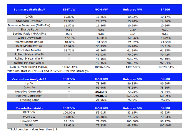
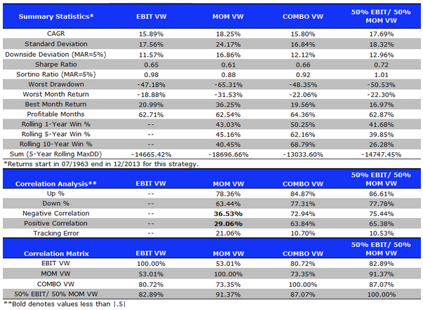
Another type of market risk that is often present in an investment portfolio is correlation risk.  This is the risk that your investment portfolio correlates to some other asset or investment index.  Such risks are often occluded – hidden from view – only to emerge when least wanted.  For example, it might be supposed that a “dollar-neutral” portfolio, i.e. a portfolio comprising equity long and short positions of equal dollar value, might be uncorrelated with the broad equity market indices.  It might well be.  On the other hand, the portfolio might become correlated with such indices during times of market turbulence; or it might correlate positively with some sector indices and negatively with others; or with market volatility, as measured by the CBOE VIX index, for instance.

Where such dependencies are included by design, they are not a problem;  but when they are unintended and latent in the investment portfolio, they often create difficulties.  The key here is to test for such dependencies against a variety of risk factors that are likely to be of concern.  These might include currency and interest rate risk factors, for example;  sector indices; or commodity risk factors such as oil or gold (in a situation where, for example, you are investing a a portfolio of mining stocks).  Once an unwanted correlation is identified, the next step is to adjust the portfolio holdings to try to eliminate it.  Typically, this can often only be done in the average, meaning that, while there is no correlation bias over the long term, there may be periods of positive, negative, or alternating correlation over shorter time horizons.  Either way, it’s important to know.

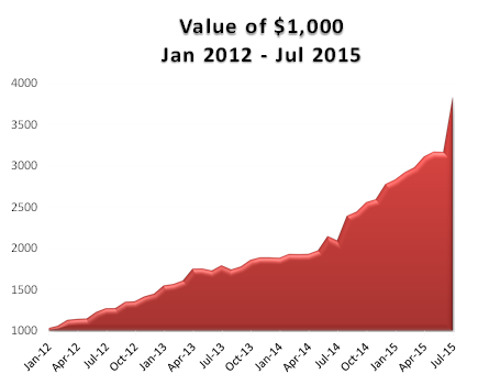
Using the Strategic Volatility Strategy as an example, we target to maximize the Sortino Ratio, subject also to maintaining very lows levels of correlation to the principal risk factors of concern to us, the S&P 500 and VIX indices. Our aim is to create a portfolio that is broadly impervious to changes in the level of the overall market, or in the level of market volatility.


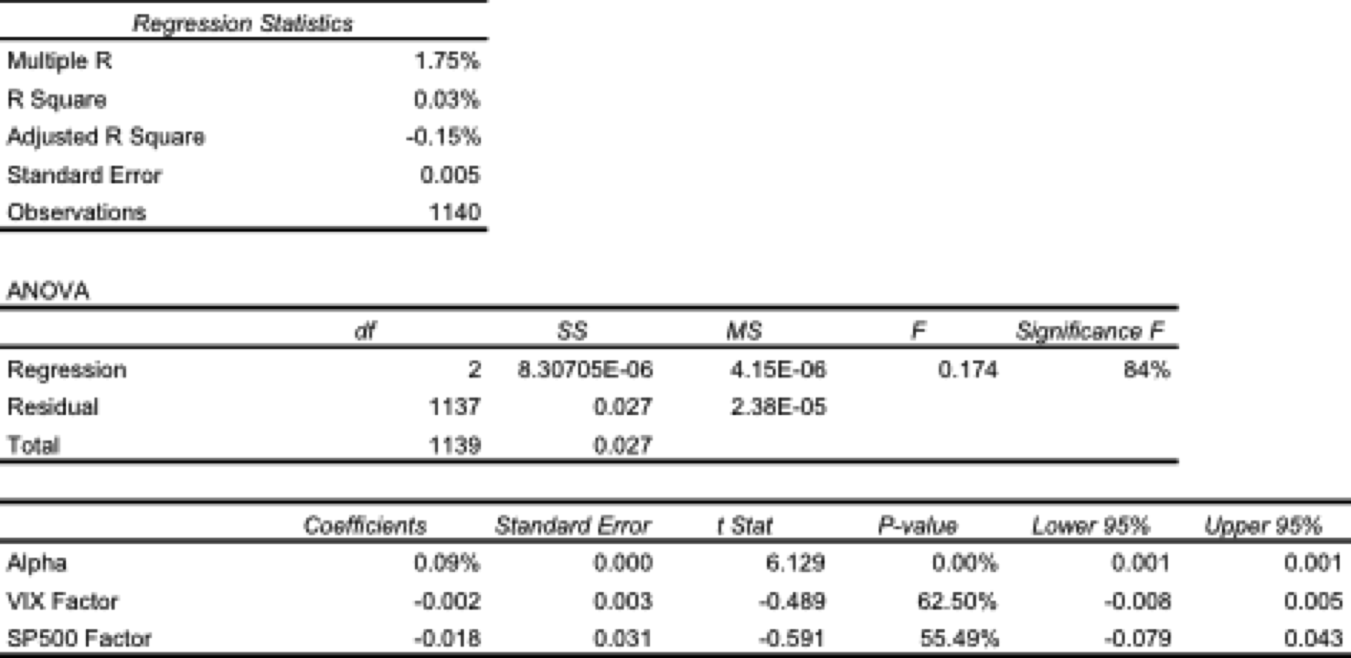
One method of quantifying such dependencies is with linear regression analysis.  By way of illustration, in the table below are shown the results of regressing the daily returns from the Strategic Volatility Strategy against the returns in the VIX and S&P 500 indices.  Both factor coefficients are statistically indistinguishable from zero, i.e. there is significant no (linear) dependency.  However, the constant coefficient, referred to as the strategy alpha, is both positive and statistically significant.  In simple terms, the strategy produces a return that is consistently positive, on average, and which is not dependent on changes in the level of the broad market, or its volatility.  By contrast, for example, a commonplace volatility strategy that entails capturing the VIX futures roll would show a negative correlation to the VIX index and a positive dependency on the S&P500 index.

Regression


Tail Risk

Ever since the publication of Nassim Taleb’s “The Black Swan”, investors have taken a much greater interest in the risk of extreme events.  If the bursting of the tech bubble in 2000 was not painful enough, investors surely appear to have learned the lesson thoroughly after the financial crisis of 2008.  But even if investors understand the concept, the question remains: what can one do about it?

The place to start is by looking at the fundamental characteristics of the portfolio returns.  Here we are not such much concerned with risk, as measured by the second moment, the standard deviation. Instead, we now want to consider the third and forth moments of the distribution, the skewness and kurtosis.

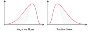
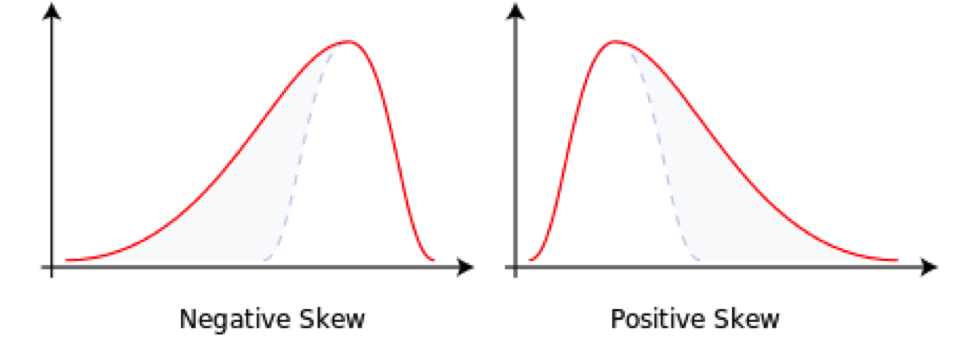
Comparing the two distributions below, we can see that the distribution on the left, with negative skew, has nonzero probability associated with events in the extreme left of the distribution, which in this context, we would associate with negative returns.  The distribution on the right, with positive skew, is likewise “heavy-tailed”; but in this case the tail “risk” is associated with large, positive returns.  That’s the kind of risk most investors can live with.


skewness


Source: Wikipedia


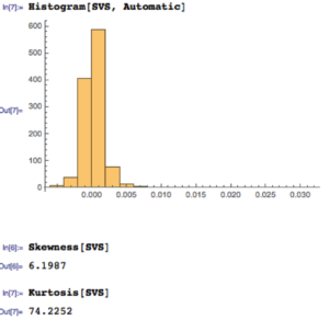
A more direct measure of tail risk is kurtosis, literally, “heavy tailed-ness”, indicating a propensity for extreme events to occur.  Again, the shape of the distribution matters:  a heavy tail in the right hand portion of the distribution is fine;  a heavy tail on the left (indicating the likelihood of large, negative returns) is a no-no.

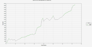
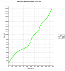
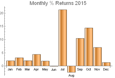
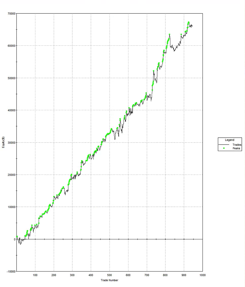
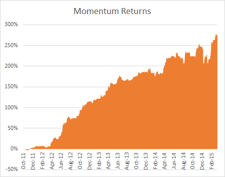
Let’s take a look at the distribution of returns for the Strategic Volatility Strategy.  As you can see, the distribution is very positively skewed, with a very heavy right hand tail.  In other words, the strategy has a tendency to produce extremely positive returns. That’s the kind of tail risk investors prefer.

SVS


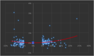
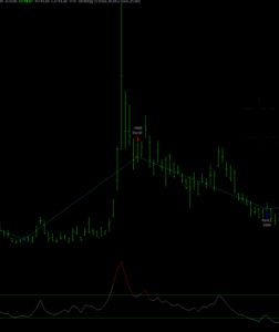
Another way to evaluate tail risk is to examine directly the performance of the strategy during extreme market conditions, when the market makes a major move up or down. Since we are using a volatility strategy as an example, let’s take a look at how it performs on days when the VIX index moves up or down by more than 5%.  As you can see from the chart below, by and large the strategy returns on such days tend to be positive and, furthermore, occasionally the strategy produces exceptionally high returns.


Convexity


The property of producing higher returns to the upside and lower losses to the downside (or, in this case, a tendency to produce positive returns in major market moves in either direction) is known as positive convexity.


Positive convexity, more typically found in fixed income portfolios, is a highly desirable feature, of course.  How can it be achieved?    Those familiar with options will recognize the convexity feature as being similar to the concept of option Gamma and indeed, one way to produce such a payoff is buy adding options to the investment mix:  put options to give positive convexity to the downside, call options to provide positive convexity to the upside (or using a combination of both, i.e. a straddle).


In this case we achieve positive convexity, not by incorporating options, but through a judicious choice of leveraged ETFs, both equity and volatility, for example, the ProShares UltraPro S&P500 ETF (NYSEArca:UPRO) and the ProShares Ultra VIX Short-Term Futures ETN (NYSEArca:UVXY).


Putting It All Together

While we have talked through the various concepts in creating a risk-protected portfolio one-at-a-time, in practice we use nonlinear optimization techniques to construct a portfolio that incorporates all of the desired characteristics simultaneously. This can be a lengthy and tedious procedure, involving lots of trial and error.  And it cannot be emphasized enough how important the choice of the investment universe is from the outset.  In this case, for instance, it would likely be pointless to target an overall positively convex portfolio without including one or more leveraged ETFs in the investment mix.

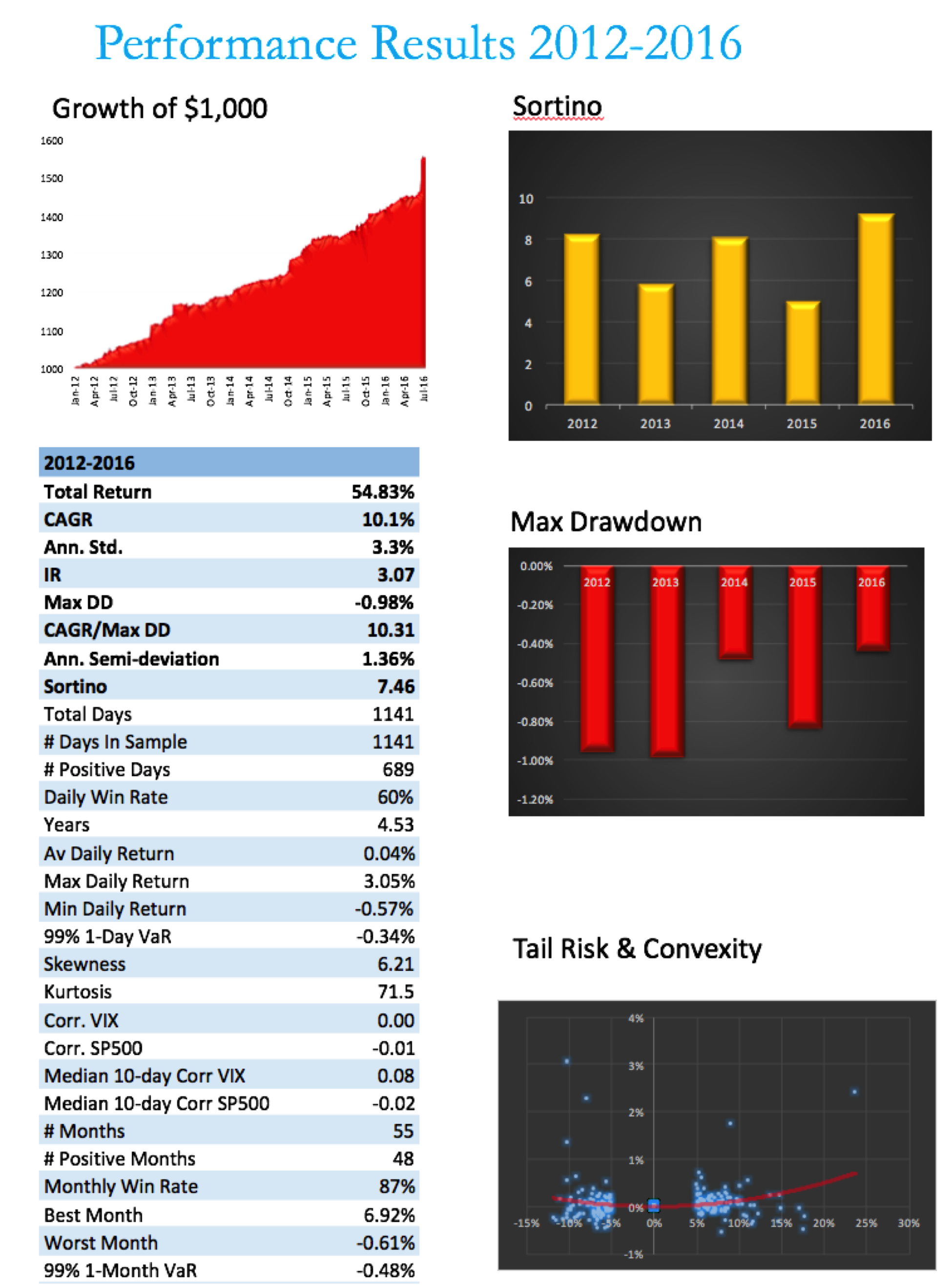
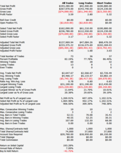
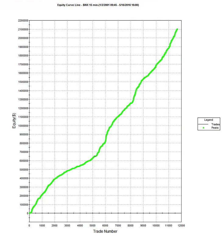
Let’s see how it turned out in the case of the Strategic Volatility Strategy.


SVS Perf


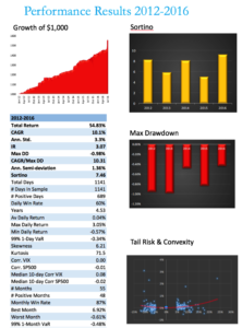
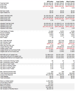
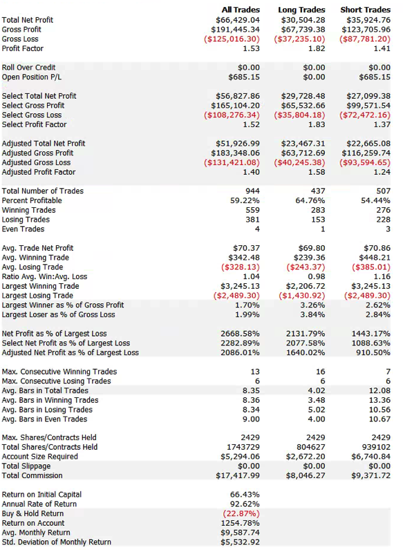
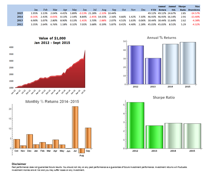
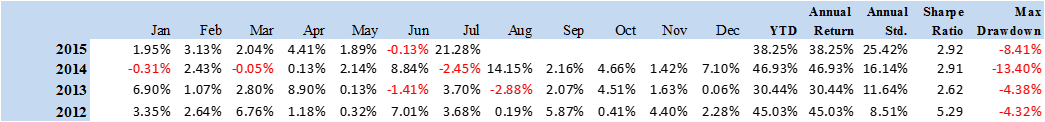
Note that, while the portfolio Information Ratio is moderate (just above 3), the Sortino Ratio is consistently very high, averaging in excess of 7.  In large part that is due to the exceptionally low downside risk, which at 1.36% is less than half the standard deviation (which is itself quite low at 3.3%).  It is no surprise that the maximum drawdown over the period from 2012 amounts to less than 1%.

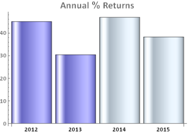
A critic might argue that a CAGR of only 10% is rather modest, especially since market conditions have generally been so benign.  I would answer that criticism in two ways.  Firstly, this is an investment that has the risk characteristics of a low-duration government bond; and yet it produces a yield many times that of a typical bond in the current low interest rate environment.

Secondly, I would point out that these results are based on use of standard 2:1 Reg-T leverage. In practice it is entirely feasible to increase the leverage up to 4:1, which would produce a CAGR of around 20%.  Investors can choose where on the spectrum of risk-return they wish to locate the portfolio and the strategy leverage can be adjusted accordingly.


Conclusion

The current investment environment, characterized by low yields and growing downside risk, poses difficult challenges for investors.  A way to address these concerns is to focus on metrics of downside risk in the construction of the investment portfolio, aiming for high Sortino Ratios, low correlation with market risk factors, and positive skewness and convexity in the portfolio returns process.

Such desirable characteristics can be achieved with modern portfolio construction techniques providing the investment universe is chosen carefully and need not include anything more exotic than a collection of commonplace ETF products.

Trading With Indices

In this post I want to discuss ways to make use of signals from relevant market indices in your trading.  These signals can add value regardless of whether you trade algorithmically or manually.  The techniques described here are one of the most widely applicable in the quantitative analyst’s arsenal.

Let’s motivate the discussion by looking an example of a simple trading system trading the VIX on weekly bars.  Performance results for the system are summarized in the chart and table below.  The system outperforms the buy and hold return by a substantial margin, with a profit factor of over 3 and a win rate exceeding 82%.  What’s not to like?

VIX EC

VIX Performance

Well, for one thing, this isn’t really a trading system – because the VIX Index itself isn’t tradable. So the performance results are purely notional (and, if you didn’t already notice, no slippage or commission is included).

It is very easy to build high-performing trading system in indices – because they are not traded products,  index prices are often stale and tend to “follow” the price action in the equivalent traded market.

This particular system for the VIX Index took me less than ten minutes to develop and comprises only a few lines of code.  The system makes use of a simple RSI indicator to decide when to buy or sell the index.  I optimized the indicator parameters (separately for long and short) over the period to 2012, and tested it out-of-sample on the data from 2013-2016.

inputs:
Price( Close ) ,
Length( 14 ) ,
OverSold( 30 ) ;

variables:
RSIValue( 0 );

RSIValue = RSI( Price, Length );
if CurrentBar > 1 and RSIValue crosses over OverSold then
Buy ( !( “RsiLE” ) ) next bar at market;

.

The daily system I built for the S&P 500 Index is a little more sophisticated than the VIX model, and produces the following results.

SP500 EC

SP500 Perf


Using Index Trading Systems

We have seen that its trivially easy to build profitable trading systems for index products.  But since they can’t be traded, what’s the point?

The analyst might be tempted by the idea of using the signals generated by an index trading system to trade a corresponding market, such as VIX or eMini futures.  However, this approach is certain to fail.  Index prices lag the prices of equivalent futures products, where traders first monetize their view on the market.  So using an index strategy directly to trade a cash or futures market would be like trying to trade using prices delayed by a few seconds, or minutes – a recipe for losing money.

SSALGOTRADING AD

Nor is it likely that a trading system developed for an index product will generalize to a traded market.  What I mean by this is that if you were to take an index strategy, such as the VIX RSI strategy, transfer it to VIX futures and tweak the parameters in the hope of producing a profitable system, you are likely to be disappointed. As I have shown, you can produce a profitable index trading system using the simplest and most antiquated trading concepts (such as the RSI index) that long ago ceased to offer any predictive value in actual traded markets.  Index markets are actually inefficient – the prices of index products often fail to fully reflect all relevant, available information in a timely way. Such simple inefficiencies are easily revealed by indicators such as moving averages.  Traded markets, by contrast, are highly efficient and, with the exception of HFT, it is going to take a great deal more than a simple moving average to provide insight into the few inefficiencies that do arise.

bullbear

Strategies in index products are best thought of, not as trading strategies, but rather as a means of providing broad guidance as to the general condition of the market and its likely direction over the longer term.  To take the VIX index strategy as an example, you can see that each “trade” spans several weeks.  So one might regard a “buy” signal from the VIX index system as an indication that volatility is expected to rise over the next month or two.  A trader might use that information to lean on the side of being long volatility, perhaps even avoiding any short volatility positions altogether for the next several weeks.  Following the model’s guidance in that way would would certainly have helped many equity and volatility traders during the market sell off during August 2015, for example:


Vix Example

The S&P 500 Index model is one I use to provide guidance as to market conditions for the current trading day.  It is a useful input to my thinking as to how aggressive I want my trading models to be during the upcoming session. If the index model suggests a positive tone to the market, with muted volatility, I might be inclined to take a more aggressive stance.  If the model starts trading to the short side, however, I am likely to want to be much more cautious.    Yesterday (May 16, 2016), for example, the index model took an early long trade, providing confirmation of the positive tenor to the market and encouraging me to trade volatility to the short side more aggressively.


SP500 Example


In general, I would tend to classify index trading systems as “decision support” tools that provide a means of shading opinion on the market, or perhaps providing a means of calibrating trading models to the anticipated market conditions. However, they can be used in a more direct way, short of actual trading.  For example, one of our volatility trading systems uses the trading signals from a trading system designed for the VVIX volatility-of-volatility index.  Another approach is to use the signals from an index trading system as an indicator of the market regime in a regime switching model.

Designing Index Trading Models

Whereas it is profitability that is typically the primary design criterion for an actual trading system, given the purpose of an index trading system there are other criteria that are at least as important.

It should be obvious from these few illustrations that you want to design your index model to trade less frequently than the system you are intending to trade live: if you are swing-trading the eminis on daily bars, it doesn’t help to see 50 trades a day from your index system.  What you want is an indication as to whether the market action over the next several days is likely to be positive or negative.  This means that, typically, you will design your index system using bar frequencies at least as long as for your live system.

Another way to slow down the signals coming from your index trading system is to design it for very high accuracy – a win rate of  70%, or higher.  It is actually quite easy to do this:  I have systems that trade the eminis on daily bars that have win rates of over 90%.  The trick is simply that you have to be prepared to wait a long time for the trade to come good.  For a live system that can often be a problem – no-one like to nurse an underwater position for days or weeks on end.  But for an index trading system it matters far less and, in fact, it helps:  because you want trading signals over longer horizons than the time intervals you are using in your live trading system.

Since the index system doesn’t have to trade live, it means of course that the usual trading costs and frictions do not apply.  The advantage here is that you can come up with concepts for trading systems that would be uneconomic in the real world, but which work perfectly well in the frictionless world of index trading.  The downside, however, is that this might lead you to develop index systems that trade far too frequently.  So, even though they should not apply, you might seek to introduce trading costs in order to penalize higher frequency trading systems and benefit systems that trade less frequently.

Designing index trading systems in an area in which genetic programming algorithms excel.  There are two main reasons for this.  Firstly, as I have previously discussed, simple technical indicators of the kind employed by GP modeling systems work well in index markets.  Secondly, and more importantly, you can use the GP system to tailor an index trading system to meet the precise criteria you have in mind, such as the % win rate, trading frequency, etc.

An outstanding product that I can highly recommend in this context is Mike Bryant’s Adaptrade Builder.  Builder is a superb piece of software whose power and ease of use reflects Mike’s engineering background and systems development expertise.


Adaptrade


ETFs vs. Hedge Funds – Why Not Combine Both?

Grace Kim, Brand Director at DarcMatter, does a good job of setting out the pros and cons of ETFs vs hedge funds for the family office investor in her LinkedIn post.

She points out that ETFs now offer as much liquidity as hedge funds, both now having around $2.96 trillion in assets.  So, too, are her points well made about the low cost, diversification and ease of investing in ETFs compared to hedge funds.

But, of course, the point of ETF investing is to mimic the return in some underlying market – to gain beta exposure, in the jargon – whereas hedge fund investing is all about alpha – the incremental return that is achieved over and above the return attributable to market risk factors.

SSALGOTRADING AD

But should an investor be forced to choose between the advantages of diversification and liquidity of ETFs on the one hand and the (supposedly) higher risk-adjusted returns of hedge funds, on the other?  Why not both?

Diversified Long/Short ETF Strategies

In fact, there is nothing whatever to prevent an investment strategist from constructing a hedge fund strategy using ETFs.  Just as one can enjoy the hedging advantages of a long/short equity hedge fund portfolio, so, too, can one employ the same techniques to construct long/short ETF portfolios.  Compared to a standard equity L/S portfolio, an ETF L/S strategy can offer the added benefit of exposure to (or hedge against) additional risk factors, including currency, commodity or interest rate.

For an example of this approach ETF long/short portfolio construction, see my post on Developing Long/Short ETF Strategies.  As I wrote in that article:

My preference for ETFs is due primarily to the fact that  it is easier to achieve a wide diversification in the portfolio with a more limited number of securities: trading just a handful of ETFs one can easily gain exposure, not only to the US equity market, but also international equity markets, currencies, real estate, metals and commodities.

More Exotic Hedge Fund Strategies with ETFs

But why stop at vanilla long/short strategies?  ETFs are so varied in terms of the underlying index, leverage and directional bias that one can easily construct much more sophisticated strategies capable of tapping the most obscure sources of alpha.

Take our very own Volatility ETF strategy for example.  The strategy constructs hedged positions, not by being long/short, but by being short/short or long/long volatility and inverse volatility products, like SVXY and UVXY, or VXX and XIV.  The strategy combines not only strategic sources of alpha that arise from factors such as convexity in the levered ETF products, but also short term alpha signals arising from temporary misalignments in the relative value of comparable ETF products.  These can be exploited by tactical, daytrading algorithms of a kind more commonly applied in the context of high frequency trading.

For more on this see for example Investing in Levered ETFs – Theory and Practice.

Does the approach work?  On the basis that a picture is worth a thousand words, let me answer that question as follows:

Systematic Strategies Volatility ETF Strategy

Perf Summary Dec 2015

Conclusion

There is no reason why, in considering the menu of ETF and hedge fund strategies, it should be a case of either-or.  Investors can combine the liquidity, cost and diversification advantages of ETFs with the alpha generation capabilities of well-constructed hedge fund strategies.

How to Make Money in a Down Market

The popular VIX blog Vix and More evaluates the performance of the VIX ETFs (actually ETNs) and concludes that all of them lost money in 2015.  Yes, both long volatility and short volatility products lost money!

VIX ETP performance in 2015

Source:  Vix and More

By contrast, our Volatility ETF strategy had an exceptional year in 2015, making money in every month but one:

Monthly Pct Returns

How to Profit in a Down Market

How do you make money when every product you are trading loses money?  Obviously you have to short one or more of them.  But that can be a very dangerous thing to do, especially in a product like the VIX ETNs.  Volatility itself is very volatile – it has an annual volatility (the volatility of volatility, or VVIX) that averages around 100% and which reached a record high of 212% in August 2015.

VVIX

The CBOE VVIX Index

Selling products based on such a volatile instrument can be extremely hazardous – even in a downtrend: the counter-trends are often extremely violent, making a short position challenging to maintain.

Relative value trading is a more conservative approach to the problem.  Here, rather than trading a single product you trade a pair, or basket of them.  Your bet is that the ETFs (or stocks) you are long will outperform the ETFs you are short.  Even if your favored ETFs declines, you can still make money if the ETFs you short declines even more.

This is the basis for the original concept of hedge funds, as envisaged by Alfred Jones in the 1940’s, and underpins the most popular hedge fund strategy, equity long-short.  But what works successfully in equities can equally be applied to other markets, including volatility.  In fact, I have argued elsewhere that the relative value (long/short) concept works even better in volatility markets, chiefly because the correlations between volatility processes tend to be higher than the correlations between the underlying asset processes (see The Case for Volatility as an Asset Class).


Daytrading Volatility ETFs

ETFAs we have discussed before, there is no standard definition of high frequency trading.  For some, trading more than once or twice a day constitutes high frequency, while others regard anything less than several hundred times a session as low, or medium frequency trading.  Hence in this post I have referred to “daytrading” since we can at least agree on that description for a strategy that exits all positions by the close of the session.

HFT Trading in ETFs – Challenges and Opportunities

High frequency trading in equities and ETFs offer their own opportunities and challenges compared to futures. Amongst the opportunities we might list:

  • Arbitrage between destinations (exchanges, dark pools) where the stock is traded
  • Earning rebates from the exchanges willing to pay for order flow
  • Arbitraging news flows amongst pairs or baskets of equities

When it comes to ETFs, unfortunately, the set of possibilities is more restricted than for single names and one is often obliged to dig deeply into the basket/replication/cointegration type of approach, which can be very challenging in a high frequency context.  The risk of one leg of a multi-asset trade being left unfilled is such that one has to be willing to cross the spread to get the trade on.  Depending on the trading platform and the quality of the execution algorithms, this can make trading the strategy prohibitively expensive.

In that case you have a number of possibilities to consider.  You can simplify the trade, limit the number of stocks in the basket and hope that there is enough alpha left in the reduced strategy. You can focus on managing the trade execution sufficiently well that aggressive trading becomes necessary on relatively few occasions and you look to minimize the costs of paying the spread when they arise.  You can design strategies with higher profit factors that are able to withstand the performance drag entailed in trading aggressively.  Or you can design slower versions of the strategy where latency, fill rates and execution costs are not such critical factors.

SSALGOTRADING AD

Developing high frequency strategies in the volatility ETFs presents special challenges.  Being fairly new, the products have limited histories, which makes modeling more of a challenge.  One way to address this is to create synthetic series priced from the VIX futures, using the published methodology for constructing the ETFs.  Be warned, though, that these synthetic series are likely to inflate your backtest results since they aren’t traded instruments.

Another practical problem that crops up regularly in products like UVXY and VXX is that the broker has difficulty locating stock for short selling.  So you are limited to taking the strategy offline when that occurs, designing strategies that trade long only, or as we do, switching to other products when the ETF is unavailable to short.

Then there is the capacity issue. Despite their fast-growing popularity, volatility ETF funds are in many cases quite small, totaling perhaps a few hundred millions of dollars in AUM. You are never going to be able to construct a strategy capable of absorbing billions of dollars of investment in the ETF products alone.

Volatility and Alpha

volatilitychartFor these reasons, volatility ETFs are not a natural choice for many investment strategists.  But they do have one great advantage compared to other products:  volatility.  Volatility implies uncertainty about the true value of a security, which means that market participants can have very different views about what it is worth at any moment in time.  So the prospects for achieving competitive advantage through superior analytical methods is much greater than for a stock that hardly moves at all and on whose value everyone concurs.  Furthermore, volatility creates regular opportunities for hitting stops, and creating mini crashes or short squeezes, in which the security is temporarily under- or over-valued.  If ever there was a security offering the potential for generating alpha, it is the volatility ETF.

The volatility of the VIX ETFs is enormous, by the standards of regular stocks.  A typical stock might have an annual volatility of 30% to 60%.  The lowest level ever seen in the VVIX index series so far is 70%. To give you an idea of how extreme it can become, during the latest market swoon in August the VVIX, the volatility-of-volatility for the S&P500 index, reached over 200% a year.

A Daytrading Strategy in the VXX

So, despite the challenges and difficulties, there are very good reasons to make the attempt to develop strategies for the volatility ETF products.  My firm, Systematic Strategies, has developed several such algorithms that are combined to create a strategy that trades the volatility ETFs very successfully.  Until recently, however,  all of the sub-strategies we employ were longer term in nature, and entailed holding positions overnight.  We wanted to develop higher frequency algorithms that could react more quickly to changes in the volatility landscape.  We had to dig pretty deep into the arsenal of trading ideas to get there, but eventually we succeeded.  After six months of live trading we were ready to release the new VXX daytrading algorithm into production for our volatility ETF strategy investors.  Here’s how it looks (results are for a $100,000 account).

Fig 1 Fig 2 Fig 3

As you can see, the strategy trades up to around 10 times a day with a reasonable profit factor (1.53) and win rate of just under 60%. By itself, the strategy has a Sharpe Ratio of around 6, so it is well worth trading on its own.  But its real value (for us) emerges when it is combined in appropriate proportion with the other, lower frequency algorithms in the volatility strategy.  The additional alpha from the VXX strategy reduces the size of the loss in August and produces a substantial gain in September, taking the YTD return to just under 50%.  Returns for Oct MTD are already at 16%.

Vol Strategy perf Sept 2015


My Big Fat Greek Vacation

LEARNING TO TRUST A TRADING SYSTEM

One of the most difficult decisions to make when running a systematic trading program is SystemTradingknowing when to override the system.  During the early 2000’s when I was running the Caissa Capital fund, the models would regularly make predictions on volatility that I and our head Trader, Ron Henley, a former option trader from the AMEX, disagreed with.  Most times, the system proved to have made the correct decision. My take-away from that experience was that, as human beings, even as traders, we are not very good at pricing risk.

My second take-away was that, by and large, you are better off trusting the system, rather than second-guessing its every decision.  Of course, markets can change and systems break down; but the right approach to assessing this possibility is to use statistical control procedures to determine formally whether or not the system has broken down, rather than going through a routine period of under-performance (see:  is your strategy still working?)

GREEK LESSONS

So when the Greek crisis blew up in June my first instinct was not to start looking grexit jisawimmediately for the escape hatch.  However, as time wore on I became increasingly concerned that the risk of a Grexit or default had not abated.  Moreover, I realized that there was really nothing comparable in the data used in the development of the trading models that was in any way comparable to the scenario facing Greece, the EU and, by a process of contagion, US markets.  Very reluctantly, therefore, I came to the decision that the smart way to play the crises was from the sidelines.  So we made the decisions to go 100% to cash and waited for the crisis to subside.

A week went by. Then another.  Of course, I had written to our investors explaining what we intended to do, and why, so there were no surprises.  Nonetheless, I felt uncomfortable not making money for them.  I did my best to console myself with the principal rule of money management: first, do not lose money.  Of course we didn’t – but neither did we make much money, and ended June more or less flat.

COMEBACK

After the worst of the crisis was behind us, I was relieved to see that the models appeared almost as anxious as I was to make up for lost time.  One of the features of the system is

poker2that it makes aggressive use of leverage. Rather like an expert poker player, when it judges the odds to be in its favor, the system will increase its bet size considerably; at other times it will hunker down, play conservatively, or even exit altogether.  Consequently, the turnover in the portfolio can be large at times.  The cost of trading high volume can substantial, especially in some of the less liquid ETF products, where the bid/ask spread can amount to several cents.  So we typically aim to execute passively, looking to buy on the bid and sell on the offer, using execution algos to split our orders up and randomize them. That also makes it tougher for HFT algos to pick us off as we move into and out of our positions.

So, in July, our Greek “vacation” at an end, the system came roaring back, all guns blazing. It quickly moved into some aggressive short volatility positions to take advantage of the elevated levels in the VIX, before reversing and gong long as the index collapsed to the bottom of the monthly range.

A DOUBLE-DIGIT MONTHLY RETURN: +21.28%

The results were rather spectacular:  a return of +21.28% for the month, bringing the totalMonthly Pct Returns return to 38.25% for 2015 YTD.

In the current low rate environment, this rate of return is extraordinary, but not entirely unprecedented: the strategy has produced double-digit monthly returns several times in the past, most recently in August last year, which saw a return of +14.1%.  Prior, to that, the record had been +8.90% in April 2013.

Such outsized returns come at a price – they have the effect of increasing strategy volatility and hence reducing the Sharpe Ratio.   Of course, investors worry far less about upside volatility than downside volatility (or simi-variance), which is why the Sortino Ratio is in some ways a more appropriate measure of risk-adjusted performance, especially for strategies like ours which has very large kurtosis.

VALUE OF $1000Since inception the compound annual growth rate (CAGR) of the strategy has been 45.60%, while the Sharpe Ratio has maintained a level of around 3 since that time.

Most of the drawdowns we have seen in the strategy have been in single digits, both in back-test and in live trading.  The only exception was in 2013, where we experienced a very short term decline of -13.40%, from which the strategy recovered with a couple of days.

In the great majority of cases, drawdowns in VIX-related strategies result from bad end-of-day “marks” in the VIX index.  These can arise for legitimate reasons, but are often

Sharpecaused by traders manipulating the index, especially around option expiration. Because of the methodology used to compute the VIX, it is very easy to move the index by 5bp to 10bp, or more, by quoting prices for deep OTM put options as expiration nears.  This can be critically important to holders of large VIX option positions and hence the temptation to engage in such manipulation may be irresistible.

For us, such market machinations are simply an annoyance, a cost of doing business in the VIX.  Sure, they inflate drawdowns and strategy volatility, but there is not much we can do about them, other wait patiently for bad “marks” to be corrected the following day, which they almost always are.

Looking ahead over the remainder of the year, we are optimistic about the strategy’s opportunities to make money in August, but, like many traders, we are apprehensive about Ann Returnsthe consequences if the Fed should decide to take action to raise rates in September.  We are likely to want to take in smaller size through the ensuing volatility, since either a long- or short-vol positions carries considerable risk in such a situation.  As and when a rate rise does occur, we anticipate a market correction of perhaps 20% or more, accompanied by surge in market volatility.  We are likely to see the VIX index reach the 20’s or 30’s, before it subsides.  However, under this scenario, opportunities to make money on the short side will likely prove highly attractive going into the final quarter of the year.  We remain hopeful of achieving a total return in the region of 40% to 50%, or more in 2015.

STRATEGY PERFORMANCE REPORT Jan 2012 – Jul 2015

Monthly Returns


The Case for Volatility as an Asset Class

Volatility as an asset class has grown up over the fifteen years since I started my first volatility arbitrage fund in 2000.  Caissa Capital grew to about $400m in assets before I moved on, while several of its rivals have gone on to manage assets in the multiple billions of dollars.  Back then volatility was seen as a niche, esoteric asset class and quite rightly so.  Nonetheless, investors who braved the unknown and stayed the course have been well rewarded: in recent years volatility strategies as an asset class have handily outperformed the indices for global macro, equity market neutral and diversified funds of funds, for example. Fig 1

The Fundamentals of Volatility

It’s worth rehearsing a few of the fundamental features of volatility for those unfamiliar with the territory.

Volatility is Unobservable

Volatility is the ultimate derivative, one whose fair price can never be known, even after the event, since it is intrinsically unobservable.  You can estimate what the volatility of an asset has been over some historical period using, for example, the standard deviation of returns.  But this is only an estimate, one of several possibilities, all of which have shortcomings.  We now know that volatility can be measured with almost arbitrary precision using an integrated volatility estimator (essentially a metric based on high frequency data), but that does not change the essential fact:  our knowledge of volatility is always subject to uncertainty, unlike a stock price, for example.

Volatility Trends

Huge effort is expended in identifying trends in commodity markets and many billions of dollars are invested in trend following CTA strategies (and, equivalently, momentum strategies in equities).  Trend following undoubtedly works, according to academic research, but is also subject to prolonged drawdowns during periods when a trend moderates or reverses. By contrast, volatility always trends.  You can see this from the charts below, which express the relationship between volatility in the S&P 500 index in consecutive months.  The r-square of the regression relationship is one of the largest to be found in economics. Fig 2 And this is a feature of volatility not just in one asset class, such as equities, nor even for all classes of financial assets, but in every time series process for which data exists, including weather and other natural phenomena.  So an investment strategy than seeks to exploit volatility trends is relying upon one of the most consistent features of any asset process we know of (more on this topic in Long Memory and Regime Shifts in Asset Volatility).

Volatility Mean-Reversion and Correlation

One of the central assumptions behind the ever-popular stat-arb strategies is that the basis between two or more correlated processes is stationary. Consequently, any departure from the long term relationship between such assets will eventually revert to the mean. Mean reversion is also an observed phenomenon in volatility processes.  In fact, the speed of mean reversion (as estimated in, say, an Ornstein-Ulenbeck framework) is typically an order of magnitude larger than for a typical stock-pairs process.  Furthermore, the correlation between one volatility process and another volatility process, or indeed between a volatility process and an asset returns process, tends to rise when markets are stressed (i.e. when volatility increases). Fig 3

Another interesting feature of volatility correlations is that they are often lower than for the corresponding asset returns processes.  One can therefore build a diversified volatility portfolio with far fewer assets that are required for, say, a basket of equities (see Modeling Asset Volatility for more on this topic).

Fig 4   Finally, more sophisticated stat-arb strategies tend to rely on cointegration rather than correlation, because cointegrated series are often driven by some common fundamental factors, rather than purely statistical ones, which may prove temporary (see Developing Statistical Arbitrage Strategies Using Cointegration for more details).  Again, cointegrated relationships tend to be commonplace in the universe of volatility processes and are typically more reliable over the long term than those found in asset return processes.

Volatility Term Structure

One of the most marked characteristics of the typical asset volatility process its upward sloping term structure.  An example of the typical term structure for futures on the VIX S&P 500 Index volatility index (as at the end of May, 2015), is shown in the chart below. A steeply upward-sloping curve characterizes the term structure of equity volatility around 75% of the time.

Fig 5   Fixed income investors can only dream of such yield in the current ZIRP environment, while f/x traders would have to plunge into the riskiest of currencies to achieve anything comparable in terms of yield differential and hope to be able to mitigate some of the devaluation risk by diversification.

The Volatility of Volatility

One feature of volatility processes that has been somewhat overlooked is the consistency of the volatility of volatility.  Only on one occasion since 2007 has the VVIX index, which measures the annual volatility of the VIX index, ever fallen below 60.

Fig 6   What this means is that, in trading volatility, you are trading an asset whose annual volatility has hardly ever fallen below 60% and which has often exceeded 100% per year.  Trading opportunities tend to abound when volatility is consistently elevated, as here (and, conversely, the performance of many hedge fund strategies tends to suffer during periods of sustained, low volatility)

SSALGOTRADING AD

Anything You Can Do, I Can Do better

The take-away from all this should be fairly obvious:  almost any strategy you care to name has an equivalent in the volatility space, whether it be volatility long/short, relative value, stat-arb, trend following or carry trading. What is more, because of the inherent characteristics of volatility, all these strategies tend to produce higher levels of performance than their more traditional counterparts. Take as an example our own Volatility ETF strategy, which has produced consistent annual returns of between 30% and 40%, with a Sharpe ratio in excess of 3, since 2012.   VALUE OF $1000

Sharpe

  Monthly Returns


(click to enlarge)

Where does the Alpha Come From?

It is traditional at this stage for managers to point the finger at hedgers as the source of abnormal returns and indeed I will do the same now.   Equity portfolio managers are hardly ignorant of the cost of using options and volatility derivatives to hedge their portfolios; but neither are they likely to be leading experts in the pricing of such derivatives.  And, after all, in a year in which they might be showing a 20% to 30% return, saving a few basis points on the hedge is neither here nor there, compared to the benefits of locking in the performance gains (and fees!). The same applies even when the purpose of using such derivatives is primarily to produce trading returns. Maple Leaf’s George Castrounis puts it this way:

Significant supply/demand imbalances continuously appear in derivative markets. The principal users of options (i.e. pension funds, corporates, mutual funds, insurance companies, retail and hedge funds) trade these instruments to express a view on the direction of the underlying asset rather than to express a view on the volatility of that asset, thus making non-economic volatility decisions. Their decision process may be driven by factors that have nothing to do with volatility levels, such as tax treatment, lockup, voting rights, or cross ownership. This creates opportunities for strategies that trade volatility.

We might also point to another source of potential alpha:  the uncertainty as to what the current level of volatility is, and how it should be priced.  As I have already pointed out, volatility is intrinsically uncertain, being unobservable.  This allows for a disparity of views about its true level, both currently and in future.  Secondly, there is no universal agreement on how volatility should be priced.  This permits at times a wide divergence of views on fair value (to give you some idea of the complexities involved, I would refer you to, for example, Range based EGARCH Option pricing Models). What this means, of course, is that there is a basis for a genuine source of competitive advantage, such as the Caissa Capital fund enjoyed in the early 2000s with its advanced option pricing models. The plethora of volatility products that have emerged over the last decade has only added to the opportunity set.

 Why Hasn’t It Been Done Before?

This was an entirely legitimate question back in the early days of volatility arbitrage. The cost of trading an option book, to say nothing of the complexities of managing the associated risks, were significant disincentives for both managers and investors.  Bid/ask spreads were wide enough to cause significant heads winds for strategies that required aggressive price-taking.  Mangers often had to juggle two sets of risks books, one reflecting the market’s view of the portfolio Greeks, the other the model view.  The task of explaining all this to investors, many of whom had never evaluated volatility strategies previously, was a daunting one.  And then there were the capacity issues:  back in the early 2000s a $400m long/short option portfolio would typically have to run to several hundred names in order to meet liquidity and market impact risk tolerances. Much has changed over the last fifteen years, especially with the advent of the highly popular VIX futures contract and the newer ETF products such as VXX and XIV, whose trading volumes and AUM are growing rapidly.  These developments have exerted strong downward pressure on trading costs, while providing sufficient capacity for at least a dozen volatility funds managing over $1Bn in assets.

Why Hasn’t It Been Done Right Yet?

Again, this question is less apposite than it was ten years ago and since that time there have been a number of success stories in the volatility space. One of the learning points occurred in 2004-2007, when volatility hit the lows for a 20 month period, causing performance to crater in long volatility funds, as well as funds with a volatility neutral mandate. I recall meeting with Nassim Taleb to discuss his Empirica volatility fund prior to that period, at the start of the 2000s.  My advice to him was that, while he had some great ideas, they were better suited to an insurance product rather than a hedge fund.  A long volatility fund might lose money month after month for an entire year, and with it investors and AUM, before seeing the kind of payoff that made such investment torture worthwhile.  And so it proved.

Conversely, stories about managers of short volatility funds showing superb performance, only to blow up spectacularly when volatility eventually explodes, are legion in this field.  One example comes to mind of a fund in Long Beach, CA, whose prime broker I visited with sometime in 2002.  He told me the fund had been producing a rock-steady 30% annual return for several years, and the enthusiasm from investors was off the charts – the fund was managing north of $1Bn by then.  Somewhat crestfallen I asked him how they were producing such spectacular returns.  “They just sell puts in the S&P, 100 points out of the money”, he told me.  I waited, expecting him to continue with details of how the fund managers handled the enormous tail risk.  I waited in vain. They were selling naked put options.  I can only imagine how those guys did when the VIX blew up in 2003 and, if they made it through that, what on earth happened to them in 2008!

Conclusion

The moral is simple:  one cannot afford to be either all-long, or all-short volatility.  The fund must run a long/short book, buying cheap Gamma and selling expensive Theta wherever possible, and changing the net volatility exposure of the portfolio dynamically, to suit current market conditions. It can certainly be done; and with the new volatility products that have emerged in recent years, the opportunities in the volatility space have never looked more promising.

Combining Momentum and Mean Reversion Strategies

The Fama-French World

For many years now the “gold standard” in factor models has been the 1996 Fama-French 3-factor model: Fig 1
Here r is the portfolio’s expected rate of return, Rf is the risk-free return rate, and Km is the return of the market portfolio. The “three factor” β is analogous to the classical β but not equal to it, since there are now two additional factors to do some of the work. SMB stands for “Small [market capitalization] Minus Big” and HML for “High [book-to-market ratio] Minus Low”; they measure the historic excess returns of small caps over big caps and of value stocks over growth stocks. These factors are calculated with combinations of portfolios composed by ranked stocks (BtM ranking, Cap ranking) and available historical market data. The Fama–French three-factor model explains over 90% of the diversified portfolios in-sample returns, compared with the average 70% given by the standard CAPM model.

The 3-factor model can also capture the reversal of long-term returns documented by DeBondt and Thaler (1985), who noted that extreme price movements over long formation periods were followed by movements in the opposite direction. (Alpha Architect has several interesting posts on the subject, including this one).

Fama and French say the 3-factor model can account for this. Long-term losers tend to have positive HML slopes and higher future average returns. Conversely, long-term winners tend to be strong stocks that have negative slopes on HML and low future returns. Fama and French argue that DeBondt and Thaler are just loading on the HML factor.

SSALGOTRADING AD

Enter Momentum

While many anomalies disappear under  tests, shorter term momentum effects (formation periods ~1 year) appear robust. Carhart (1997) constructs his 4-factor model by using FF 3-factor model plus an additional momentum factor. He shows that his 4-factor model with MOM substantially improves the average pricing errors of the CAPM and the 3-factor model. After his work, the standard factors of asset pricing model are now commonly recognized as Value, Size and Momentum.

 Combining Momentum and Mean Reversion

In a recent post, Alpha Architect looks as some possibilities for combining momentum and mean reversion strategies.  They examine all firms above the NYSE 40th percentile for market-cap (currently around $1.8 billion) to avoid weird empirical effects associated with micro/small cap stocks. The portfolios are formed at a monthly frequency with the following 2 variables:

  1. Momentum = Total return over the past twelve months (ignoring the last month)
  2. Value = EBIT/(Total Enterprise Value)

They form the simple Value and Momentum portfolios as follows:

  1. EBIT VW = Highest decile of firms ranked on Value (EBIT/TEV). Portfolio is value-weighted.
  2. MOM VW = Highest decile of firms ranked on Momentum. Portfolio is value-weighted.
  3. Universe VW = Value-weight returns to the universe of firms.
  4. SP500 = S&P 500 Total return

The results show that the top decile of Value and Momentum outperformed the index over the past 50 years.  The Momentum strategy has stronger returns than value, on average, but much higher volatility and drawdowns. On a risk-adjusted basis they perform similarly. Fig 2   The researchers then form the following four portfolios:

  1. EBIT VW = Highest decile of firms ranked on Value (EBIT/TEV). Portfolio is value-weighted.
  2. MOM VW = Highest decile of firms ranked on Momentum. Portfolio is value-weighted.
  3. COMBO VW = Rank firms independently on both Value and Momentum.  Add the two rankings together. Select the highest decile of firms ranked on the combined rankings. Portfolio is value-weighted.
  4. 50% EBIT/ 50% MOM VW = Each month, invest 50% in the EBIT VW portfolio, and 50% in the MOM VW portfolio. Portfolio is value-weighted.

With the following results:

Fig 3 The main takeaways are:

  • The combined ranked portfolio outperforms the index over the same time period.
  • However, the combination portfolio performs worse than a 50% allocation to Value and a 50% allocation to Momentum.

A More Sophisticated Model

Yangru Wu of Rutgers has been doing interesting work in this area over the last 15 years, or more. His 2005 paper (with Ronald Balvers), Momentum and mean reversion across national equity markets, considers joint momentum and mean-reversion effects and allows for complex interactions between them. Their model is of the form Fig 4 where the excess return for country i (relative to the global equity portfolio) is represented by a combination of mean-reversion and autoregressive (momentum) terms. Balvers and Wu  find that combination momentum-contrarian strategies, used to select from among 18 developed equity markets at a monthly frequency, outperform both pure momentum and pure mean-reversion strategies. The results continue to hold after corrections for factor sensitivities and transaction costs. The researchers confirm that momentum and mean reversion occur in the same assets. So in establishing the strength and duration of the momentum and mean reversion effects it becomes important to control for each factor’s effect on the other. The momentum and mean reversion effects exhibit a strong negative correlation of 35%. Accordingly, controlling for momentum accelerates the mean reversion process, and controlling for mean reversion may extend the momentum effect.

 Momentum, Mean Reversion and Volatility

The presence of  strong momentum and mean reversion in volatility processes provides a rationale for the kind of volatility strategy that we trade at Systematic Strategies.  One  sophisticated model is the Range Based EGARCH model of  Alizadeh, Brandt, and Diebold (2002) .  The model posits a two-factor volatility process in which a short term, transient volatility process mean-reverts to a stochastic long term mean process, which may exhibit momentum, or long memory effects  (details here).

In our volatility strategy we model mean reversion and momentum effects derived from the level of short and long term volatility-of-volatility, as well as the forward volatility curve. These are applied to volatility ETFs, including levered ETF products, where convexity effects are also important.  Mean reversion is a well understood phenomenon in volatility, as, too, is the yield roll in volatility futures (which also impacts ETF products like VXX and XIV).

Momentum effects are perhaps less well researched in this context, but our research shows them to be extremely important.  By way of illustration, in the chart below I have isolated the (gross) returns generated by one of the momentum factors in our model.

Fig 6