The SABR Stochastic Volatility Model

The SABR (Stochastic Alpha, Beta, Rho) model is a stochastic volatility model, which attempts to capture the volatility smile in derivatives markets. The name stands for “Stochastic Alpha, Beta, Rho”, referring to the parameters of the model. The model was developed by Patrick Hagan, Deep Kumar, Andrew Lesniewski, and Diana Woodward.

The-SABR-Stochastic-Volatility-Model

The Hedged Volatility Strategy

Being short regular Volatility ETFs or long Inverse Volatility ETFs are winning strategies…most of the time. The challenge is that when the VIX spikes or when the VIX futures curve is downward sloping instead of upward sloping, very significant losses can occur. Many people have built and back-tested models that attempt to move from long to short to neutral positions in the various Volatility ETFs, but almost all of them have one or both of these very significant flaws: 1) Failure to use “out of sample” back-testing and 2) Failure to protect against “black swan” events.

In this strategy a position and weighting in the appropriate Volatility ETFs are established based on a multi-factor model which always uses out of sample back-testing to determine effectiveness. Volatility Options are always used to protect against significant short-term moves which left unchecked could result in the total loss of one’s portfolio value; these options will usually lose money, but that is a small price to pay for the protection they provide. (Strategies should be scaled at a minimum of 20% to ensure options protection.)

This is a good strategy for IRA accounts in which short selling is not allowed. Long positions in Inverse Volatility ETFs are typically held. Suggested minimum capital: $26,000 (using 20% scaling).

Covered Writes, Covered Wrongs

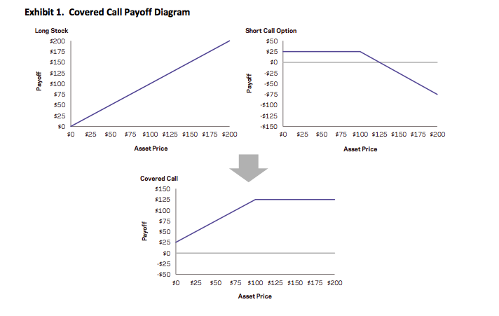
What is a Covered Call?

covered call (or covered write or buy-write) is a long position in a security and a short position in a call option on that security.  The diagram below constructs the covered call payoff diagram, including the option premium, at expiration when the call option is written at a $100 strike with a $25 option premium.

Payoff

Equity index covered calls are an attractive strategy to many investors because they have realized returns not much lower than those of the equity market but with much lower volatility.  But investors often do the trade for the wrong reasons:  there are a number of myths about covered writes that persist even amongst professional options traders.  I have heard most, if not all of them professed by seasons floor traders on the American Stock Exchange and, I confess, I have even used one or two of them myself.  Roni Israelov and Larn Nielsen of AQR Capital Management, LLC have done a fine job of elucidating and then dispelling these misunderstandings about the strategy, in their paper Covered Call Strategies: One Fact and Eight Myths, Financial Analysts Journal, Vol. 70, No. 6, 2014.

SSALGOTRADING AD

The Cover Call Strategy and its Benefits for Investors

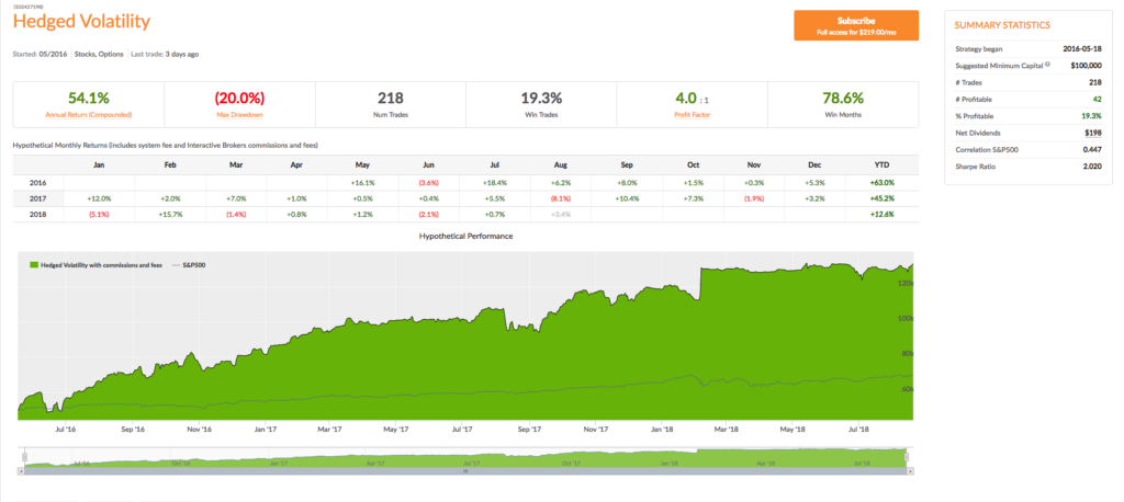
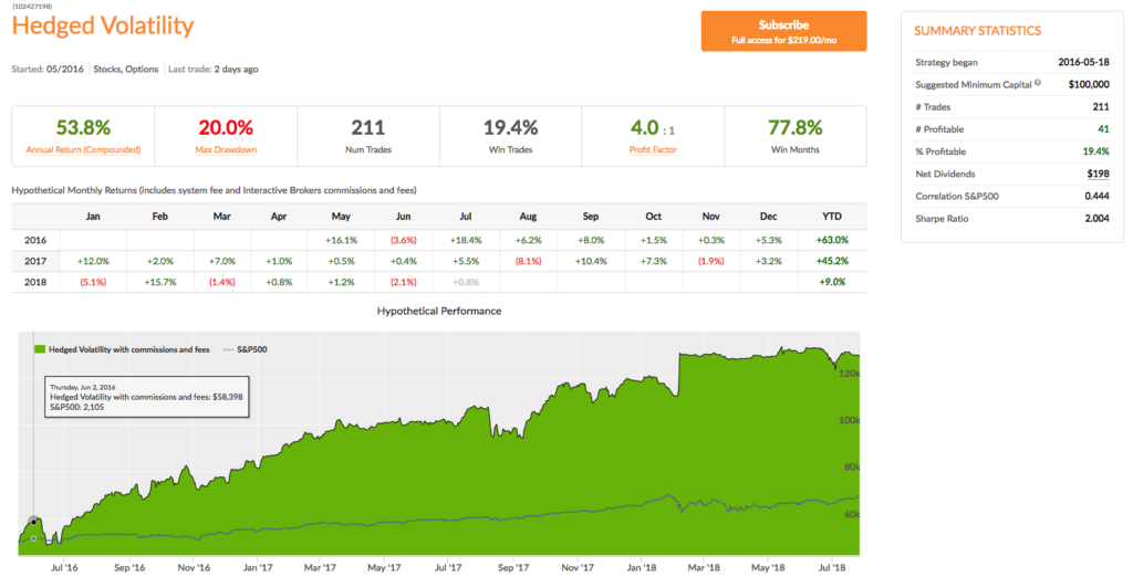
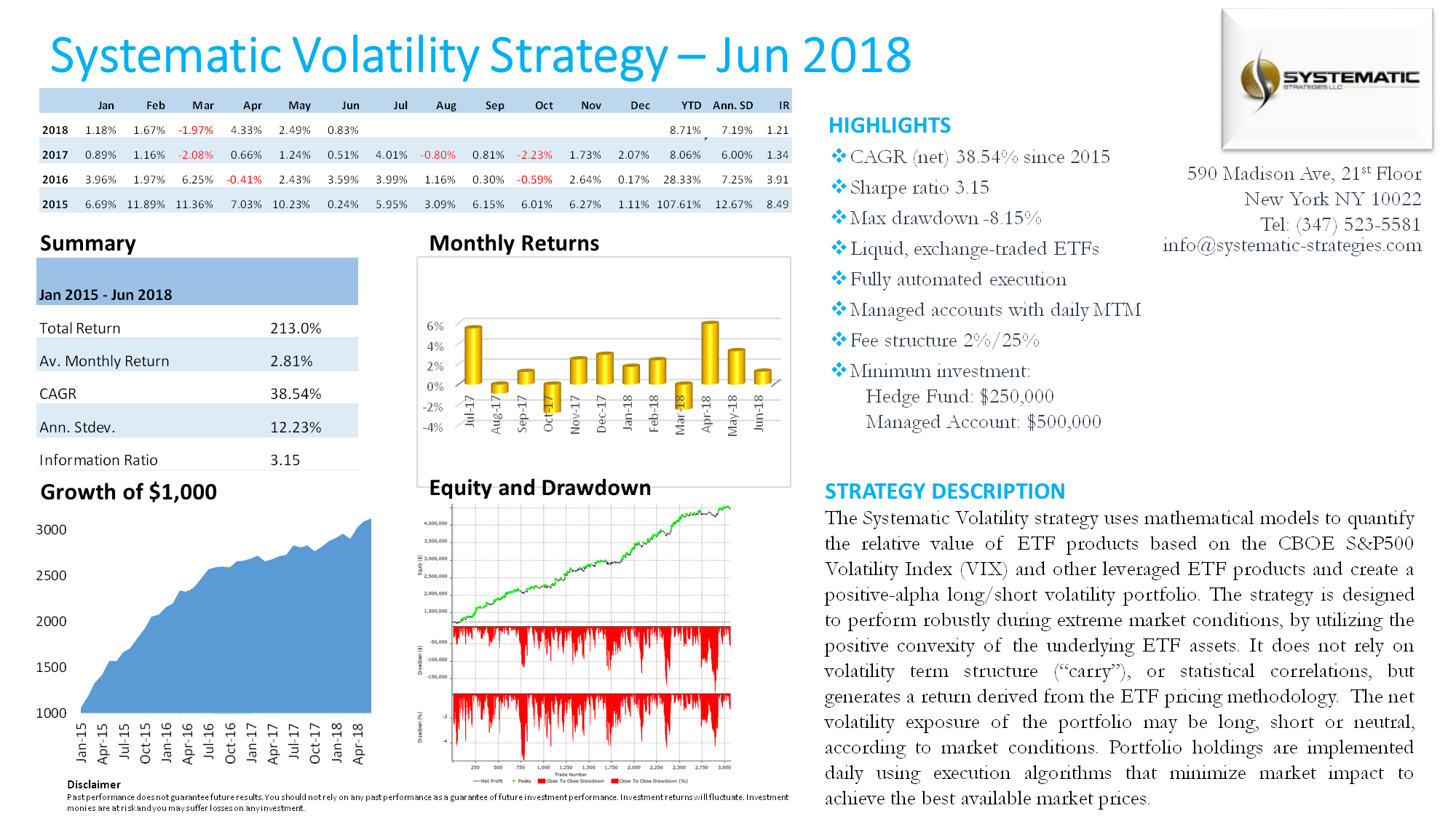
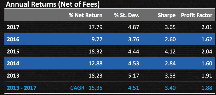
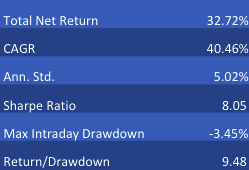
The covered call strategy has generated attention due to its attractive historical risk-adjusted returns. For example, the CBOE S&P 500 BuyWrite Index, the industry-standard covered call benchmark, is commonly described as providing average returns comparable to the S&P 500 Index with approximately two-thirds the volatility, supported by statistics such as those shown below.

Table 1

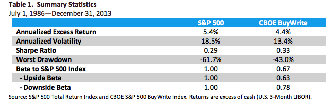
The key advantages of the strategy (compared to an outright, delta-one position) include lower volatility, beta and tail risk.  As a consequence, the strategy produces higher risk-adjusted rates if return (Sharpe Ratio).  Note, too, the beta convexity of the strategy, a topic I cover in this post:

http://jonathankinlay.com/2017/05/beta-convexity/

Although the BuyWrite Index has historically demonstrated similar total returns to the S&P 500, it does so with a reduced beta to the S&P 500 Index. However, it is important to also understand that the BuyWrite Index is more exposed to negative S&P 500 returns than positive returns. This asymmetric relationship to the S&P 500 is consistent with its payoff characteristics and results from the fact that a covered call strategy sells optionality. What this means in simple terms is that while drawdowns are somewhat mitigated by the revenue associated with call writing, the upside is capped by those same call options.

Understandably, a strategy that produces equity-like return with lower beta and lower risk attracts considerable attention from investors.  According to Moringstar, growth in assets under management in covered call strategies has been over 25% per year over the 10 years through June 2014 with over $45 billion currently invested.

Myths about the Covered Call Strategy

Many option strategies are the subject of investor myths, partly, I suppose, because option strategies are relatively complicated and entail risks in several dimensions.  So it is quite easy for investors to become confused.  Simple anecdotes are attractive because they appear to cut through the complexity with an easily understood metaphor, but they can often be misleading.  An example is the widely-held view – even amongst professional option traders – is that selling volatility via strangles is a less risk approach than selling at-the-money straddles. Intuitively, this makes sense:  why wouldn’t  selling straddles that have strike prices (far) away from the current spot price be less risky than selling straddles that have strike prices close to the spot price?  But, in fact, it turns out that selling straddles is the less risky the two strategies – see this post for details:

http://jonathankinlay.com/2016/11/selling-volatility/

Likewise, the covered call strategy is subject to a number of “urban myths”, that turn out to be unfounded:

Myth 1: Risk exposure is described by the payoff diagram

That is only true at expiration.  Along the way, the positions will be marked-to-market and may produce a substantially different payoff if the trade is terminated early.  The same holds true for a zero-coupon bond – we know the terminal value for certain, but there can be considerable variation in the value of the asset from day to day.

Myth 2: Covered calls provide downside protection

This is partially true, but only in a very limited sense.  Unlike a long option hedge, the “protection” in a buy-write strategy is limited to only the premium collected on the option sale, a relatively modest amount in most cases.  Consider a covered call position on a $100 stock with a $10 at-the-money call premium. The covered call can potentially lose $90 and the long call option can lose $10. Each position has the same 50% exposure to the stock, but the covered call’s downside risk is disproportionate to its stock exposure. This is consistent with the covered call’s realized upside and downside betas as discussed earlier.

Myth 3: Covered calls generate income.

Remember that income is revenue minus costs.

It is true that option selling generates positive cash flow, but this incorrectly leads investors to the conclusion that covered calls generate investment income.  Just as is the case with bond issuance, the revenue generated from selling the call option is not income (though, like income, the cash flows received from selling options are considered taxable for many investors). In order for there to be investment income or earnings, the option must be sold at a favorable price – the option’s implied volatility needs to be higher than the stock’s expected volatility.

Myth 4: Covered calls on high-volatility stocks and/or shorter-dated options provide higher yield.

Though true that high volatility stocks and short-dated options command higher annualized premiums, insurance on riskier assets should rationally command a higher premium and selling insurance more often per year should provide higher annual premiums. However, these do not equate to higher net income or yield. For instance, if options are properly priced (e.g., according to the Black-Scholes pricing model), then selling 12 at-the-money options will generate approximately 3.5 times the cash flow of selling a single annual option, but this does not unequivocally translate into higher net profits as discussed earlier. Assuming fairly priced options, higher revenue is not necessarily a mechanism for increasing investment income.

The key point here is that what matters is value, not price. In other words, expected investment profits are generated by the option’s richness, not the option’s price. For example, if you want to short a stock with what you consider to be a high valuation, then the goal is not to find a stock with a high price, but rather one that is overpriced relative to its fundamental value. The same principle applies to options. It is not appropriate to seek an option with a high price or other characteristics associated with high prices. Investors must instead look for options that are expensive relative to their fundamental value.  Put another way, the investor should seek out options trading at a higher implied volatility than the likely futures realized volatility over the life of the option.

Myth 5: Time decay of options written works in your favor.

While it is true that the value of an option declines over time as it approaches expiration, that is not the whole story.  In fact an option’s expected intrinsic value increases as the underlying security realizes volatility.  What matters is whether the realized volatility turns out to be lower than the volatility baked into the option price – the implied volatility.  In truth, an option’s time decay only works in the seller’s favor if the option is initially priced expensive relative to its fundamental value. If the option is priced cheaply, then time decay works very much against the seller.

Myth 6: Covered calls are appropriate if you have a neutral to moderately bullish view.

This myth is an over-simplification.  In selling a call option you are expressing a view, not only on the future prospects for the stock, but also on its likely future volatility.  It is entirely possible that the stock could stall (or even decline) and yet the value of the option you have sold rises due, say, to takeover rumors.  A neutral view on the stock may imply a belief that the security price will not move far from its current price rather than its expected return is zero. If so, then a short straddle position is a way to express that view — not a covered call — because, in this case, no active position should be taken in the security.

Myth 7: Overwriting pays you for doing what you were going to do anyway

This myth is typically posed as the following question: if you have a price target for selling a stock you own, why not get paid to write a call option struck at that price target?

In fact this myth exposes the critical difference between a plan and a contractual obligation. If the former case, suppose that the stock hits your target price very much more quickly than you had anticipated, perhaps as a result of a new product announcement that you had not anticipated at the time you set your target.  In those circumstances you might very well choose to maintain your long position and revise your price target upwards. This is an example of a plan – a successful one – that can be adjusted to suit circumstances as they change.

A covered call strategy is an obligation, rather than a plan.  You have pre-sold the stock at the target price and, in the above scenario, you cannot change your mind in order to benefit from additional potential upside in the stock.

In other words, with a covered call strategy you have monetized the optionality that is inherent in any plan and turned it into a contractual obligation in exchange for a fee.

Myth 8: Overwriting allows you to buy a stock at a discounted price.

Here is how this myth is typically framed: if a stock that you would like to own is currently priced at $100 and that you think is currently expensive, you can act on that opinion by selling a naked put option at a $95 strike price and collect a premium of say $1. Then, if the price subsequently declines below the strike price, the option will likely be exercised thus requiring you to buy the stock for $95. Including the $1 premium, you effectively buy the stock at a 6% discount. If the option is not exercised you keep the premium as income. So, this type of outcome for selling naked put options may also lead you to conclude that the equivalent covered call strategy makes sense and is valuable.

But this argument is really a sleight of hand.  In our example above, if the option is exercised, then when you buy the stock for $95 you won’t care what the stock price was when you sold the option. What matters is the stock price on the date the option was exercised. If the stock price dropped all the way down to $80, the $95 purchase price no longer seems like a discount. Your P&L will show a mark-to-market loss of $14 ($95 – $80 – $1). The initial stock price is irrelevant and the $1 premium hardly helps.

Conclusion: How to Think About the Covered Call Strategy

Investors should ignore the misleading storytelling about obtaining downside buffers and generating income. A covered call strategy only generates income to the extent that any other strategy generates income, by buying or selling mispriced securities or securities with an embedded risk premium. Avoid the temptation to overly focus on payoff diagrams. If you believe the index will rise and implied volatilities are rich, a covered call is a step in the right direction towards expressing that view.

If you have no view on implied volatility, there is no reason to sell options, or covered calls

Aby znaleźć legalne kasyna online w Polsce, odwiedź stronę pl.kasynopolska10.com/legalne-kasyna/, partnera serwisu recenzującego kasyna online – KasynoPolska10.

Using Volatility to Predict Market Direction

Decomposing Asset Returns


We can decompose the returns process Rt as follows:

While the left hand side of the equation is essentially unforecastable, both of the right-hand-side components of returns display persistent dynamics and hence are forecastable. Both the signs of returns and magnitude of returns are conditional mean dependent and hence forecastable, but their product is conditional mean independent and hence unforecastable. This is an example of a nonlinear “common feature” in the sense of Engle and Kozicki (1993).

Although asset returns are essentially unforecastable, the same is not true for asset return signs (i.e. the direction-of-change). As long as expected returns are nonzero, one should expect sign dependence, given the overwhelming evidence of volatility dependence. Even in assets where expected returns are zero, sign dependence may be induced by skewness in the asset returns process.  Hence market timing ability is a very real possibility, depending on the relationship between the mean of the asset returns process and its higher moments. The highly nonlinear nature of the relationship means that conditional sign dependence is not likely to be found by traditional measures such as signs autocorrelations, runs tests or traditional market timing tests. Sign dependence is likely to be strongest at intermediate horizons of 1-3 months, and unlikely to be important at very low or high frequencies. Empirical tests demonstrate that sign dependence is very much present in actual US equity returns, with probabilities of positive returns rising to 65% or higher at various points over the last 20 years. A simple logit regression model captures the essentials of the relationship very successfully.

Now consider the implications of dependence and hence forecastability in the sign of asset returns, or, equivalently, the direction-of-change. It may be possible to develop profitable trading strategies if one can successfully time the market, regardless of whether or not one is able to forecast the returns themselves.  

There is substantial evidence that sign forecasting can often be done successfully. Relevant research on this topic includes Breen, Glosten and Jaganathan (1989), Leitch and Tanner (1991), Wagner, Shellans and Paul (1992), Pesaran and Timmerman (1995), Kuan and Liu (1995), Larsen and Wozniak (10050, Womack (1996), Gencay (1998), Leung Daouk and Chen (1999), Elliott and Ito (1999) White (2000), Pesaran and Timmerman (2000), and Cheung, Chinn and Pascual (2003).

There is also a huge body of empirical research pointing to the conditional dependence and forecastability of asset volatility. Bollerslev, Chou and Kramer (1992) review evidence in the GARCH framework, Ghysels, Harvey and Renault (1996) survey results from stochastic volatility modeling, while Andersen, Bollerslev and Diebold (2003) survey results from realized volatility modeling.

Sign Dynamics Driven By Volatility Dynamics

Let the returns process Rt be Normally distributed with mean m and conditional volatility st.

The probability of a positive return Pr[Rt+1 >0] is given by the Normal CDF F=1-Prob[0,f]


For a given mean return, m, the probability of a positive return is a function of conditional volatility st. As the conditional volatility increases, the probability of a positive return falls, as illustrated in Figure 1 below with m = 10% and st = 5% and 15%.

In the former case, the probability of a positive return is greater because more of the probability mass lies to the right of the origin. Despite having the same, constant expected return of 10%, the process has a greater chance of generating a positive return in the first case than in the second. Thus volatility dynamics drive sign dynamics.  

 Figure 1

Email me at jkinlay@investment-analytics.com.com for a copy of the complete article.


Volatility Trading Styles

The VIX Surge of Feb 2018

Volatility trading has become a popular niche in investing circles over the last several years.  It is easy to understand why:  with yields at record lows it has been challenging to find an alternative to equities that offers a respectable return.  Volatility, however, continues to be volatile (which is a good thing in this context) and the steepness of the volatility curve has offered investors attractive returns by means of the volatility carry trade.  In this type of volatility trading the long end of the vol curve is sold, often using longer dated futures in the CBOE VIX Index, for example.  The idea is that profits are generated as the contract moves towards expiration, “riding down” the volatility curve as it does so.  This is a variant of the ever-popular “riding down the yield curve” strategy, a staple of fixed income traders for many decades.  The only question here is what to use to hedge the short volatility exposure – highly correlated S&P500 futures are a popular choice, but the resulting portfolio is exposed to significant basis risk.  Besides, when the volatility curve flatten and inverts, as it did in spectacular fashion in February, the transition tends to happen very quickly, producing a substantial losses on the portfolio.  These may be temporary, if the volatility spike is small or short-lived, but as traders and investors discovered in the February drama, neither of these two desirable outcomes is guaranteed.  Indeed as I pointed out in an earlier post this turned out to be the largest ever two-day volatility surge in history.  The results for many hedge funds, especially in the quant sector were devastating, with several showing high single digit or double-digit losses for the month.

VIX_Spike_1


Over time, investors have become more familiar with the volatility space and have learned to be wary of strategies like volatility carry or option selling, where the returns look superficially attractive, until a market event occurs.  So what alternative approaches are available?

An Aggressive Approach to Volatility Trading

In my blog post Riders on the Storm  I described one such approach:  the Option Trader strategy on our Algo Trading Platform made a massive gain of 27% for the month of February and as a result strategy performance is now running at over 55% for 2018 YTD, while maintaining a Sharpe Ratio of 2.23.

Option Trader


The challenge with this style of volatility trading is that it requires a trader (or trading system) with a very strong stomach and an investor astute enough to realize that sizable drawdowns are in a sense “baked in” for this trading strategy and should be expected from time to time.  But traders are often temperamentally unsuited to this style of trading – many react by heading for the hills and liquidating positions at the first sign of trouble; and the great majority of investors are likewise unable to withstand substantial drawdowns, even if the eventual outcome is beneficial.

SSALGOTRADING AD

The Market Timing Approach

So what alternatives are there?  One way of dealing with the problem of volatility spikes is simply to try to avoid them.  That means developing a strategy logic that step aside altogether when there is a serious risk of an impending volatility surge.  Market timing is easy to describe, but very hard to implement successfully in practice.  The VIX Swing Trader strategy on the Systematic Algotrading platform attempts to do just that, only trading when it judges it safe to do so. So, for example, it completely side-stepped the volatility debacle in August 2015, ending the month up +0.74%.  The strategy managed to do the same in February this year, finishing ahead +1.90%, a pretty creditable performance given how volatility funds performed in general.  One helpful characteristic of the strategy is that it trades the less-volatile mid-section of the volatility curve, in the form of the VelocityShares Daily Inverse VIX MT ETN (ZIV).  This ensures that the P&L swings are much less dramatic than for strategies exposed to the front end of the curve, as most volatility strategies are.

VIX Swing Trader1 VIX Swing Trader2

A potential weakness of the strategy is that it will often miss great profit opportunities altogether, since its primary focus is to keep investors out of trouble. Allied to this, the system may trade only a handful of times each month.  Indeed, if you look at the track record above you find find months in which the strategy made no trades at all. From experience, investors are almost as bad at sitting on their hands as they are at taking losses:  patience is not a highly regarded virtue in the investing community these days.  But if you are a cautious, patient investor looking for a source of uncorrelated alpha, this strategy may be a good choice. On the other hand, if you are looking for high returns and are willing to take the associated risks, there are choices better suited to your goals.

The Hedging Approach to Volatility Trading

A “middle ground” is taken in our Hedged Volatility strategy. Like the VIX Swing Trader this strategy trades VIX ETFs/ETNs, but it does so across the maturity table. What distinguishes this strategy from the others is its use of long call options in volatility products like the iPath S&P 500 VIX ST Futures ETN (VXX) to hedge the short volatility exposure in other ETFs in the portfolio.  This enables the strategy to trade much more frequently, across a wider range of ETF products and maturities, with the security of knowing that the tail risk in the portfolio is protected.  Consequently, since live trading began in 2016, the strategy has chalked up returns of over 53% per year, with a Sharpe Ratio of 2 and Sortino Ratio above 3.  Don’t be confused by the low % of trades that are profitable:  the great majority of these loss-making “trades” are in fact hedges, which one would expect to be losers, as most long options trades are.  What matters is the overall performance of the strategy.

Hedged Volatility

All of these strategies are available on our Systematic Algotrading Platform, which offers investors the opportunity to trade the strategies in their own brokerage account for a monthly subscription fee.

The Multi-Strategy Approach

The approach taken by the Systematic Volatility Strategy in our Systematic Strategies hedge fund again seeks to steer a middle course between risk and return.  It does so by using a meta-strategy approach that dynamically adjusts the style of strategy deployed as market conditions change.  Rather than using options (the strategy’s mandate includes only ETFs) the strategy uses leveraged ETFs to provide tail risk protection in the portfolio. The strategy has produced an average annual compound return of 38.54% since live trading began in 2015, with a Sharpe Ratio of 3.15:

Systematic Volatility Strategy 1 Page Tear Sheet June 2018


A more detailed explanation of how leveraged ETFs can be used in volatility trading strategies is given in an earlier post:

http://jonathankinlay.com/2015/05/investing-leveraged-etfs-theory-practice/


Conclusion:  Choosing the Investment Style that’s Right for You

There are different styles of volatility trading and the investor should consider carefully which best suits his own investment temperament.  For the “high risk” investor seeking the greatest profit the Option Trader strategy in an excellent choice, producing returns of +176% per year since live trading began in 2016.   At the other end of the spectrum, the VIX Swing trader is suitable for an investor with a cautious trading style, who is willing to wait for the right opportunities, i.e. ones that are most likely to be profitable.  For investors seeking to capitalize on opportunities in the volatility space, but who are concerned about the tail risk arising from major market corrections, the Hedge Volatility strategy offers a better choice.  Finally, for investors able to invest $250,000 or more, a hedge fund investment in our Systematic Volatility strategy offers the highest risk-adjusted rate of return.

Riders on the Storm

The Worst Volatility Scare for Years

February 2018 was an insane month for stocks, wrote CNN:

A profound inflation scare. Not one but two 1,000-point plunges for the Dow. And a powerful comeback that almost went straight back up.

The CNN story-line continues:

The Dow plummeted more than 3,200 points, or 12%, in just two weeks. Then stocks raced back to life, at one point recovering about three-quarters of those losses.

Fittingly, February ended with more drama. The Dow tumbled 680 points during the month’s final two days, leaving it down about 1,600 points from the record high in late January.

The headline in the Financial Times was a little more nuanced, focusing on the impact of the market turmoil on quant hedge funds:


FT


Quant Funds Get Trashed

The FT reported:

Computer-driven, trend-following hedge funds are heading for their worst month in nearly 17 years after getting whipsawed when the stock market’s steady soar abruptly reversed into one of the quickest corrections in history earlier in February.

The carnage amongst hedge funds was widespread, according to the article:

Société Générale’s CTA index is down 5.55 per cent this month, even after the recent market rebound, making it the worst period for these systematic hedge funds since November 2001.
Man AHL’s $1.1bn Diversified fund lost almost 10 per cent in the month to February 16, while the London investment firm’s AHL Evolution and Alpha funds were down about 4-5 per cent over the same period. The flagship funds of GAM’s Cantab Capital, Systematica and Winton lost 9.5 per cent, 7.2 per cent and 4.6 per cent* respectively between the start of the month and February 16. Aspect Capital’s Diversified Fund dropped 9.5 per cent in the month to February 20, while a trend-following fund run by Lynx Asset Management slumped 12.7 per cent. A leveraged version of the same fund tumbled 18.8 per cent. One of the other big victims is Roy Niederhoffer, whose fund lost 21.1 per cent in the month to February 20.

Painful reading, indeed.


Traders conditioned to a state of somnambulance were shocked by the ferocity of the volatility spike, as the CBOE VIX index soared by over 200% in a single day, reaching a high of over 38 on Feb 5th:


VIX Index


Indeed, this turned out to be the largest ever two-day increase in the history of the index:

VIX_Spike_1

This Quant Strategy Made 27% In February Alone

So, for a quant-driven options strategy that is typically a premium seller, February must surely have been a disaster, if not a total wipe-out.  Not quite.  On the contrary, our Option Trader strategy made a massive gain of 27% for the month.  As a result strategy performance is now running at over 55% for 2018 YTD, while maintaining a Sharpe Ratio of 2.23.

Option Trader

You can tell that the strategy has a tendency to collect option premiums, not only because the strategy description says as much, but also from the observation that over 90% of strategy trades have been profitable – one of the defining characteristics of volatility strategies that are short-Vega, long-Theta.  The theory is that such strategies make money most of the time, but then give it all back (and more) when volatility inevitably spikes.  While that is generally true, in my experience, that clearly didn’t occur here.  So what’s the story?

One of the advantages of our Algo Trading Platform is that it not only reports in detail the live performance of our strategies, but it also reveals the actual trades on the site (typically delayed by 24-72 hours).  A review of the trades made by the Option Trader strategy from the end of January though early February indicates a strongly bullish bias, with short put trades in stocks such as Netflix, Inc. (NFLX), Shopify Inc. (SHOP), The Goldman Sachs Group, Inc. (GS) and Facebook, Inc. (FB), coupled with short call trades in VIX ETF products such as ProShares Ultra VIX Short-Term Futures (UVXY) and iPath S&P 500 VIX ST Futures ETN (VXX).  As volatility began to spike on 2/5, more calls were sold at increasingly fat premiums in several of the VIX Index ETFs.  These short volatility positions were later hedged with long trades in the underlying ETFs and, over time, both the hedges and the original option sales proved highly profitable. In other words, the extremely high levels of volatility enabled the strategy to profit on both legs of the trade, a highly unusual occurrence.  Meanwhile, while it was hedging its bets in the VIX ETF option trades, the strategy was becoming increasingly aggressive in the single stocks sector, taking outright long positions in Baidu, Inc. (BIDU), Align Technology, Inc. (ALGN), Netflix, Inc. (NFLX) and others, just as they became trading off their lows in the second week of the month.  By around Feb 12th the strategy recognized that the volatility shock had begun to subside and took advantage of the inflated option premia, selling puts across the board, in particular in the technology (Tesla, Inc. (TSLA), NVIDIA Corporation (NVDA)) and retail sectors (GrubHub Inc. (GRUB), Alibaba Group Holding Limited (BABA)) that had suffered especially heavy declines.  Many of these trades were closed at a substantial profit within a span of just a few days as the market stabilized and volatility subsided.  The strategy broadened the scope of its option selling as the month progressed, initially recovering the entirety of the drawdown it had initially suffered, before going on to register substantial profits on almost every trade.

To summarize:

  1.  Like many other market players, the Volatility Trader strategy was initially caught on the wrong side of the volatility spike and suffered a significant drawdown.
  2. Instead of liquidating positions, the strategy began hedging aggressively in sectors holding the greatest danger – VIX ETFs, in particular.  These trades ultimately proved profitable on both option and hedge legs as the market turned around and volatility collapsed.
  3. As soon as volatility showed signed of easing, the strategy began making aggressive bets on market stabilization and recovery, taking long positions in some of the most beaten-down stocks and selling puts across the board to capture inflated option premia.

Lesson Learned:  Aggressive Defense is the best Options Strategy in a Volatile Market

If there is one lesson above all others to be learned from this case study it is this:  that a period of market turmoil is a time of opportunity for option traders, but only if they play aggressively, both in defense and offense.  Many traders run scared at times like this and liquidate positions, taking heavy losses in the process that can prove impossible to recover from if, as here, the drawdown is severe.  This study shows that by holding one’s nerve and hedging rather than liquidating loss-making positions and then moving aggressively to capitalize on inflated option prices a trader can not only weather the storm but, as in this case, produce exceptional returns.

The key take-away is this: in order to play aggressively you have to have sufficient reserves in the tank to enable you to hold positions rather than liquidate them and, later on, to transition to selling expensive option premiums.  The mistake many option traders make is to trade too close to the line in term of margin limits, resulting  in a forced liquidation of positions that would otherwise have been profitable.

You can trade the Option Trader strategy live in your own brokerage account – go here for details.


Finding Alpha in 2018

Given the current macro-economic environment, where should investors focus their search for sources of alpha in the year ahead?  By asking enough economists or investment managers you will find as many different opinions on the subject as would care to, no doubt many of them conflicting.  These are some thoughts on the subject from my perspective, as a quantitative hedge fund manager.

SSALGOTRADING AD

Global Market Performance in 2017

Let’s begin by reviewing some of the best and worst performing assets of 2017 (I am going to exclude cryptocurrencies from the ensuing discussion).  Broadly speaking, the story across the piste has been one of strong appreciation in emerging markets, both in equities and currencies, especially in several of the Eastern European economies.  In Government bond markets Greece has been the star of the show, having stepped back from the brink of the economic abyss.  Overall, international diversification has been a key to investment success in 2017 and I believe that pattern will hold in 2018.

BestWorstEquityMkts2017

BestWorstCurrencies2017

BestWorstGvtBond


US Yield Curve and Its Implications

Another key development that investors need to take account of is the extraordinary degree of flattening of the yield curve in US fixed income over the course of 2017:

YieldCurve


This process has now likely reached the end point and will begin to reverse as the Fed and other central banks in developed economies start raising rates.  In 2018 investors should seek to protect their fixed income portfolios by shortening duration, moving towards the front end of the curve.

US Volatility and Equity Markets

A prominent feature of US markets during 2017 has been the continuing collapse of equity index volatility, specifically the VIX Index, which reached an all-time low of 9.14 in November and continues to languish at less than half the average level of the last decade:

VIX Index

Source: Wolfram Alpha

One consequence of the long term decline in volatility has been to drastically reduce the profitability of derivatives markets, for both traders and market makers. Firms have struggled to keep up with the high cost of technology and the expense of being connected to the fragmented U.S. options market, which is spread across 15 exchanges. Earlier in 2017, Interactive Brokers Group Inc. sold its Timber Hill options market-making unit — a pioneer of electronic trading — to Two Sigma Securities.   Then, in November, Goldman Sachs announced it was shuttering its option market making business in US exchanges, citing high costs, sluggish volume and low volatility.

The impact has likewise been felt by volatility strategies, which performed well in 2015 and 2016, only to see returns decline substantially in 2017.  Our own Systematic Volatility strategy, for example, finished the year up only 8.08%, having produced over 28% in the prior year.

One side-effect of low levels of index volatility has been a fall in stock return correlations, and, conversely, a rise in the dispersion of stock returns.   It turns out that index volatility and stock correlation are themselves correlated and indeed, cointegrated:

http://jonathankinlay.com/2017/08/correlation-cointegration/


In simple terms, stocks have a tendency to disperse more widely around an increasingly sluggish index.  The “kinetic energy” of markets has to disperse somewhere and if movements in the index are muted then relative movement in individual equity returns will become more accentuated.  This is an environment that ought to favor stock picking and both equity long/short and market neutral strategies  should outperform.  This certainly proved to be the case for our Quantitative Equity long/short strategy, which produced a net return of 17.79% in 2017, but with an annual volatility of under 5%:

QE Perf


Looking ahead to 2018, I expect index volatility and equity correlations rise as  the yield curve begins to steepen, producing better opportunities for volatility strategies.  Returns from equity long/short and market neutral strategies may moderate a little as dispersion diminishes.

Futures Markets

Big increases in commodity prices and dispersion levels also lead to improvements in the performance of many CTA strategies in 2017. In the low frequency space our Futures WealthBuilder strategy produced a net return of 13.02% in 2017, with a Sharpe Ratio above 3 (CAGR from inception in 2013 is now at 20.53%, with an average annual standard deviation of 6.36%).  The star performer, however, was our High Frequency Futures strategy.  Since launch in March 2017 this has produce a net return of 32.72%, with an annual standard deviation of 5.02%, on track to generate an annual Sharpe Ratio above 8 :

HFT Perf

Looking ahead, the World Bank has forecast an increase of around 4% in energy prices during 2018, with smaller increases in the price of agricultural products.   This is likely to be helpful to many CTA strategies, which will likely see further enhancements in performance over the course of the year.  Higher frequency strategies are more dependent on commodity market volatility, which is seen more likely to rise than fall in the year ahead.

Conclusion

US fixed income investors are likely to want to shorten duration as the yield curve begins to steepen in 2018, bringing with it higher levels of index volatility that will favor equity high frequency and volatility strategies.  As in 2017, there is likely much benefit to be gained in diversifying across international equity and currency markets.  Strengthening energy prices are likely to sustain higher rates of return in futures strategies during the coming year.

Correlation Copulas

Continuing a previous post, in which we modeled the relationship in the levels of the VIX Index and the Year 1 and Year 2 CBOE Correlation Indices, we next turn our attention to modeling changes in the VIX index.

In case you missed it, the post can be found here:

http://jonathankinlay.com/2017/08/correlation-cointegration/

We saw previously that the levels of the three indices are all highly correlated, and we were able to successfully account for approximately half the variation in the VIX index using either linear regression models or non-linear machine-learning models that incorporated the two correlation indices.  It turns out that the log-returns processes are also highly correlated:

Fig1 Fig2

A Linear Model of VIX Returns

We can create a simple linear regression model that relates log-returns in the VIX index to contemporaneous log-returns in the two correlation indices, as follows.  The derived model accounts for just under 40% of the variation in VIX index returns, with each correlation index contributing approximately one half of the total VIX return.

SSALGOTRADING AD

Fig3

Non-Linear Model of VIX Returns

Although the linear model is highly statistically significant, we see clear evidence of lack of fit in the model residuals, which indicates non-linearities present in the relationship.  So, ext we use a nearest-neighbor algorithm, a machine learning technique that allows us to model non-linear components of the relationship.  The residual plot from the nearest neighbor model clearly shows that it does a better job of capturing these nonlinearities, with lower standard in the model residuals, compared to the linear regression model:

Fig4

Correlation Copulas

Another approach entails the use of copulas to model the inter-dependency between the volatility and correlation indices.  For a fairly detailed exposition on copulas, see the following blog posts:

http://jonathankinlay.com/2017/01/copulas-risk-management/


http://jonathankinlay.com/2017/03/pairs-trading-copulas/

We begin by taking a smaller sample comprising around three years of daily returns in the indices.  This minimizes the impact of any long-term nonstationarity in the processes and enables us to fit marginal distributions relatively easily.  First, let’s look at the correlations in our sample data:

Fig5

We next proceed to fit margin distributions to the VIX and Correlation Index processes.  It turns out that the VIX process is well represented by a Logistic distribution, while the two Correlation Index returns processes are better represented by a Student-T density.  In all three cases there is little evidence of lack of fit, wither in the body or tails of the estimated probability density functions:

Fig6 Fig7 Fig8

The final step is to fit a copula to model the joint density between the indices.  To keep it simple I have chosen to carry out the analysis for the combination of the VIX index with only the first of the correlation indices, although in principle there no reason why a copula could not be estimated for all three indices.  The fitted model is a multinormal Gaussian copula with correlation coefficient of 0.69.  of course, other copulas are feasible (Clayton, Gumbel, etc), but Gaussian model appears to provide an adequate fit to the empirical copula, with approximate symmetry in the left and right tails.

Fig9


Modeling Volatility and Correlation

In a previous blog post I mentioned the VVIX/VIX Ratio, which is measured as the ratio of the CBOE VVIX Index to the VIX Index. The former measures the volatility of the VIX, or the volatility of volatility.

http://jonathankinlay.com/2017/07/market-stress-test-signals-danger-ahead/

A follow-up article in ZeroHedge shortly afterwards pointed out that the VVIX/VIX ratio had reached record highs, prompting Goldman Sachs analyst Ian Wright to comment that this could signal the ending of the current low-volatility regime:

vvix to vix 2_0


A linkedIn reader pointed out that individual stock volatility was currently quite high and when selling index volatility one is effectively selling stock correlations, which had now reached historically low levels. I concurred:

What’s driving the low vol regime is the exceptionally low level of cross-sectional correlations. And, as correlations tighten, index vol will rise. Worse, we are likely to see a feedback loop – higher vol leading to higher correlations, further accelerating the rise in index vol. So there is a second order, Gamma effect going on. We see that is the very high levels of the VVIX index, which shot up to 130 last week. The all-time high in the VVIX prior to Aug 2015 was around 120. The intra-day high in Aug 2015 reached 225. I’m guessing it will get back up there at some point, possibly this year.

SSALGOTRADING AD

As there appears to be some interest in the subject I decided to add a further blog post looking a little further into the relationship between volatility and correlation.  To gain some additional insight we are going to make use of the CBOE implied correlation indices.  The CBOE web site explains:

Using SPX options prices, together with the prices of options on the 50 largest stocks in the S&P 500 Index, the CBOE S&P 500 Implied Correlation Indexes offers insight into the relative cost of SPX options compared to the price of options on individual stocks that comprise the S&P 500.

  • CBOE calculates and disseminates two indexes tied to two different maturities, usually one year and two years out. The index values are published every 15 seconds throughout the trading day.
  • Both are measures of the expected average correlation of price returns of S&P 500 Index components, implied through SPX option prices and prices of single-stock options on the 50 largest components of the SPX.

Dispersion Trading

One application is dispersion trading, which the CBOE site does a good job of summarizing:

The CBOE S&P 500 Implied Correlation Indexes may be used to provide trading signals for a strategy known as volatility dispersion (or correlation) trading. For example, a long volatility dispersion trade is characterized by selling at-the-money index option straddles and purchasing at-the-money straddles in options on index components. One interpretation of this strategy is that when implied correlation is high, index option premiums are rich relative to single-stock options. Therefore, it may be profitable to sell the rich index options and buy the relatively inexpensive equity options.

The VIX Index and the Implied Correlation Indices

Again, the CBOE web site is worth quoting:

The CBOE S&P 500 Implied Correlation Indexes measure changes in the relative premium between index options and single-stock options. A single stock’s volatility level is driven by factors that are different from what drives the volatility of an Index (which is a basket of stocks). The implied volatility of a single-stock option simply reflects the market’s expectation of the future volatility of that stock’s price returns. Similarly, the implied volatility of an index option reflects the market’s expectation of the future volatility of that index’s price returns. However, index volatility is driven by a combination of two factors: the individual volatilities of index components and the correlation of index component price returns.

Let’s dig into this analytically.  We first download and plot the daily for the VIX and Correlation Indices from the CBOE web site, from which it is evident that all three series are highly correlated:

Fig1

An inspection reveals significant correlations between the VIX index and the two implied correlation indices, which are themselves highly correlated.  The S&P 500 Index is, of course, negatively correlated with all three indices:

Fig8

Modeling Volatility-Correlation

The response surface that describes the relationship between the VIX index and the two implied correlation indices is locally very irregular, but the slope of the surface is generally positive, as we would expect, since the level of VIX correlates positively with that of the two correlation indices.

Fig2

The most straightforward approach is to use a simple linear regression specification to model the VIX level as a function of the two correlation indices.  We create a VIX Model Surface object using this specification with the  Mathematica Predict function:Fig3The linear model does quite a good job of capturing the positive gradient of the response surface, and in fact has a considerable amount of explanatory power, accounting for a little under half the variance in the level of the VIX index:

Fig 4

However, there are limitations.  To begin with, the assumption of independence between the explanatory variables, the correlation indices, clearly does not hold.  In cases such as this, where explanatory variables are multicolinear, we are unable to draw inferences about the explanatory power of individual regressors, even though the model as a whole may be highly statistically significant, as here.

Secondly, a linear regression model is not going to capture non-linearities in the volatility-correlation relationship that are evident in the surface plot.  This is confirmed by a comparison plot, which shows that the regression model underestimates the VIX level for both low and high values of the index:

Fig5

We can achieve a better outcome using a machine learning algorithm such as nearest neighbor, which is able to account for non-linearities in the response surface:

Fig6

The comparison plot shows a much closer correspondence between actual and predicted values of the VIX index,  even though there is evidence of some remaining heteroscedasticity in the model residuals:

Fig7

Conclusion

A useful way to think about index volatility is as a two dimensional process, with time-series volatility measured on one dimension and dispersion (cross-sectional volatility, the inverse of correlation) measured on the second.  The two factors are correlated and, as we have shown here, interact in a complicated, non-linear way.

The low levels of index volatility we have seen in recent months result, not from low levels of volatility in component stocks, but in the historically low levels of correlation (high levels of dispersion) in the underlying stock returns processes. As correlations begin to revert to historical averages, the impact will be felt in an upsurge in index volatility, compounded by the non-linear interaction between the two factors.


Market Stress Test Signals Danger Ahead

One metric of market stress is the VX Ratio, defined as the ratio of the CBOE VVIX Index to the VIX Index. The former measures the volatility of the VIX, or the volatility of volatility.  When markets are very quiet and the VIX Index is low the ratio moves to higher levels. During periods of market stress the ratio moves down as the VIX Index skyrockets.

Below we chart the daily movement in the ratio over the period from 2007, when it peaked at just over 8, before collapsing to a low of 1.3 during the financial crisis of 2008.

Fig 1


Highest Level in a Decade

During the market run-up from 2009 the VX Ratio once more climbed to nosebleed levels, exceeding the peak achieved in 2007 as the VIX Index declined to single-digit values last seen a decade ago.

A histogram of the VX Ratio shows that in only 68 out of the 3,844-day history of the series (around 1.7%) has the ratio reached the level we are seeing currently.

SSALGOTRADING AD

That said, the time series doesn’t appear to be stationary, so the ratio could continue on its upward trajectory almost indefinitely, in theory. My sense, however, is that this is unlikely to happen. Instead, I expect a significant market decline, accompanied by higher levels in the VIX index and a reversion of the VX Ratio to intermediate levels.

This isn’t a new call, of course – the general consensus appears to be that it is a matter of when, not if, we can expect a market correction. Based on the VX Ratio and other measures, such as forward P/E, the market does appear to be over-extended and likely to correct in the third quarter of 2017, as the Fed tightens further.


Fig2

Decoupling

Underpinning the concerns about the continued rally in equities is the disconnect from economic fundamentals, specifically Industrial Production, which has been moving sideways since the end of 2014 during the continued upward surge in equities.

IP


Of course, all this illustrates is that markets can remain “irrational” for longer than you can remain solvent (if you trade from the short side).

One chart that might provide a clue as to the timing of a significant market pullback is the level of short interest, which has fallen the lowest level since the market peak in 2007:

Short Interest


However, before concluding that the sky is imminently about to fall, we might take note of the fact that short interest was at even lower levels during the mid-2000’s, when market conditions were benign.  Furthermore, despite short interest declining precipitously from mid-2011 to mid-2012, the market continued serenely on its upward trajectory.   In other words, if past history is any guide, short interest could continue lower, or reverse course and trend higher, without any corresponding change in the market’s overall direction of travel.

Conclusion

All this goes to show just how difficult it is, in a post-QE world, to forecast the timing of a possible market correction.  For what it’s worth I doubt we will see a major economic slowdown, or mild recession, until late 2018. But I believe that we are likely to see escalating levels of volatility accompanied by periodic short-term market turbulence well before then.  My best guess is that we may see a repeat of the Aug 2015 downdraft later this year, in the September/October time-frame.  But if that scenarios does play out I would expect the market to recover quickly and rally into the end of the year.