Dynamic Time Warping


QUANTITATIVE RESEARCH AND TRADING
The latest theories, models and investment strategies in quantitative research and trading

LEARNING TO TRUST A TRADING SYSTEM
One of the most difficult decisions to make when running a systematic trading program is  knowing when to override the system. During the early 2000’s when I was running the Caissa Capital fund, the models would regularly make predictions on volatility that I and our head Trader, Ron Henley, a former option trader from the AMEX, disagreed with. Most times, the system proved to have made the correct decision. My take-away from that experience was that, as human beings, even as traders, we are not very good at pricing risk.
My second take-away was that, by and large, you are better off trusting the system, rather than second-guessing its every decision. Of course, markets can change and systems break down; but the right approach to assessing this possibility is to use statistical control procedures to determine formally whether or not the system has broken down, rather than going through a routine period of under-performance (see: is your strategy still working?)
GREEK LESSONS
So when the Greek crisis blew up in June my first instinct was not to start looking immediately for the escape hatch. However, as time wore on I became increasingly concerned that the risk of a Grexit or default had not abated. Moreover, I realized that there was really nothing comparable in the data used in the development of the trading models that was in any way comparable to the scenario facing Greece, the EU and, by a process of contagion, US markets. Very reluctantly, therefore, I came to the decision that the smart way to play the crises was from the sidelines. So we made the decisions to go 100% to cash and waited for the crisis to subside.
A week went by. Then another. Of course, I had written to our investors explaining what we intended to do, and why, so there were no surprises. Nonetheless, I felt uncomfortable not making money for them. I did my best to console myself with the principal rule of money management: first, do not lose money. Of course we didn’t – but neither did we make much money, and ended June more or less flat.
COMEBACK
After the worst of the crisis was behind us, I was relieved to see that the models appeared almost as anxious as I was to make up for lost time. One of the features of the system is
 that it makes aggressive use of leverage. Rather like an expert poker player, when it judges the odds to be in its favor, the system will increase its bet size considerably; at other times it will hunker down, play conservatively, or even exit altogether. Consequently, the turnover in the portfolio can be large at times. The cost of trading high volume can substantial, especially in some of the less liquid ETF products, where the bid/ask spread can amount to several cents. So we typically aim to execute passively, looking to buy on the bid and sell on the offer, using execution algos to split our orders up and randomize them. That also makes it tougher for HFT algos to pick us off as we move into and out of our positions.
So, in July, our Greek “vacation” at an end, the system came roaring back, all guns blazing. It quickly moved into some aggressive short volatility positions to take advantage of the elevated levels in the VIX, before reversing and gong long as the index collapsed to the bottom of the monthly range.
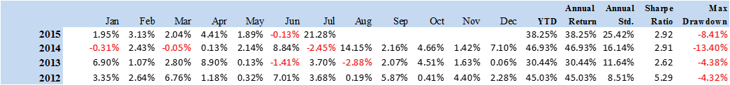
A DOUBLE-DIGIT MONTHLY RETURN: +21.28%
The results were rather spectacular: a return of +21.28% for the month, bringing the total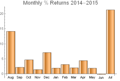 return to 38.25% for 2015 YTD.
In the current low rate environment, this rate of return is extraordinary, but not entirely unprecedented: the strategy has produced double-digit monthly returns several times in the past, most recently in August last year, which saw a return of +14.1%. Prior, to that, the record had been +8.90% in April 2013.
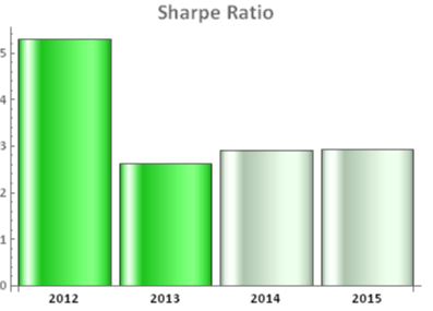
Such outsized returns come at a price – they have the effect of increasing strategy volatility and hence reducing the Sharpe Ratio. Of course, investors worry far less about upside volatility than downside volatility (or simi-variance), which is why the Sortino Ratio is in some ways a more appropriate measure of risk-adjusted performance, especially for strategies like ours which has very large kurtosis.
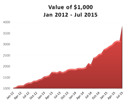 Since inception the compound annual growth rate (CAGR) of the strategy has been 45.60%, while the Sharpe Ratio has maintained a level of around 3 since that time.
Most of the drawdowns we have seen in the strategy have been in single digits, both in back-test and in live trading. The only exception was in 2013, where we experienced a very short term decline of -13.40%, from which the strategy recovered with a couple of days.
In the great majority of cases, drawdowns in VIX-related strategies result from bad end-of-day “marks” in the VIX index. These can arise for legitimate reasons, but are often
 caused by traders manipulating the index, especially around option expiration. Because of the methodology used to compute the VIX, it is very easy to move the index by 5bp to 10bp, or more, by quoting prices for deep OTM put options as expiration nears. This can be critically important to holders of large VIX option positions and hence the temptation to engage in such manipulation may be irresistible.
For us, such market machinations are simply an annoyance, a cost of doing business in the VIX. Sure, they inflate drawdowns and strategy volatility, but there is not much we can do about them, other wait patiently for bad “marks” to be corrected the following day, which they almost always are.
Looking ahead over the remainder of the year, we are optimistic about the strategy’s opportunities to make money in August, but, like many traders, we are apprehensive about 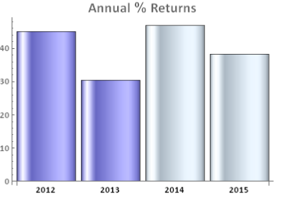 the consequences if the Fed should decide to take action to raise rates in September. We are likely to want to take in smaller size through the ensuing volatility, since either a long- or short-vol positions carries considerable risk in such a situation. As and when a rate rise does occur, we anticipate a market correction of perhaps 20% or more, accompanied by surge in market volatility. We are likely to see the VIX index reach the 20’s or 30’s, before it subsides. However, under this scenario, opportunities to make money on the short side will likely prove highly attractive going into the final quarter of the year. We remain hopeful of achieving a total return in the region of 40% to 50%, or more in 2015.
STRATEGY PERFORMANCE REPORT Jan 2012 – Jul 2015

Recently I have been working on the problem of how to construct large portfolios of cointegrated securities. My focus has been on ETFs rather that stocks, although in principle the methodology applies equally well to either, of course.
My preference for ETFs is due primarily to the fact that it is easier to achieve a wide diversification in the portfolio with a more limited number of securities: trading just a handful of ETFs one can easily gain exposure, not only to the US equity market, but also international equity markets, currencies, real estate, metals and commodities. Survivorship bias, shorting restrictions and security-specific risk are also less of an issue with ETFs than with stocks (although these problems are not too difficult to handle).
On the downside, with few exceptions ETFs tend to have much shorter histories than equities or commodities. One also has to pay close attention to the issue of liquidity. That said, I managed to assemble a universe of 85 ETF products with histories from 2006 that have sufficient liquidity collectively to easily absorb an investment of several hundreds of millions of dollars, at minimum.
The basic methodology for constructing a long/short portfolio using cointegration is covered in an earlier post. But problems arise when trying to extend the universe of underlying securities. There are two challenges that need to be overcome.

The first issue is that, other than the simple regression approach, more advanced techniques such as the Johansen test are unable to handle data sets comprising more than about a dozen securities. The second issue is that the number of possible combinations of cointegrated securities quickly becomes unmanageable as the size of the universe grows. In this case, even taking a subset of just six securities from the ETF universe gives rise to a total of over 437 million possible combinations (85! / (79! * 6!). An exhaustive test of all the possible combinations of a larger portfolio of, say, 20 ETFs, would entail examining around 1.4E+19 possibilities.
Given the scale of the computational problem, how to proceed? One approach to addressing the cardinality issue is sparse canonical correlation analysis, as described in Identifying Small Mean Reverting Portfolios, d’Aspremont (2008). The essence of the idea is something like this. Suppose you find that, in a smaller, computable universe consisting of just two securities, a portfolio comprising, say, SPY and QQQ was found to be cointegrated. Then, when extending consideration to portfolios of three securities, instead of examining every possible combination, you might instead restrict your search to only those portfolios which contain SPY and QQQ. Having fixed the first two selections, you are left with only 83 possible combinations of three securities to consider. This process is repeated as you move from portfolios comprising 3 securities to 4, 5, 6, … etc.
Other approaches to the cardinality problem are possible. In their 2014 paper Sparse, mean reverting portfolio selection using simulated annealing, the Hungarian researchers Norbert Fogarasi and Janos Levendovszky consider a new optimization approach based on simulated annealing. I have developed my own, hybrid approach to portfolio construction that makes use of similar analytical methodologies. Does it work?
Below are summarized the out-of-sample results for a portfolio comprising 21 cointegrated ETFs over the period from 2010 to 2015. The basket has broad exposure (long and short) to US and international equities, real estate, currencies and interest rates, as well as exposure in banking, oil and gas and other specific sectors.
The portfolio was constructed using daily data from 2006 – 2009, and cointegration vectors were re-computed annually using data up to the end of the prior year. I followed my usual practice of using daily data comprising “closing” prices around 12pm, i.e. in the middle of the trading session, in preference to prices at the 4pm market close. Although liquidity at that time is often lower than at the close, volatility also tends to be muted and one has a period of perhaps as much at two hours to try to achieve the arrival price. I find this to be a more reliable assumption that the usual alternative.
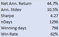
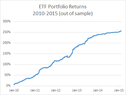 The risk-adjusted performance of the strategy is consistently outstanding throughout the out-of-sample period from 2010. After a slowdown in 2014, strategy performance in the first quarter of 2015 has again accelerated to the level achieved in earlier years (i.e. with a Sharpe ratio above 4).
Another useful test procedure is to compare the strategy performance with that of a portfolio constructed using standard mean-variance optimization (using the same ETF universe, of course). The test indicates that a portfolio constructed using the traditional Markowitz approach produces a similar annual return, but with 2.5x the annual volatility (i.e. a Sharpe ratio of only 1.6). What is impressive about this result is that the comparison one is making is between the out-of-sample performance of the strategy vs. the in-sample performance of a portfolio constructed using all of the available data.
Having demonstrated the validity of the methodology, at least to my own satisfaction, the next step is to deploy the strategy and test it in a live environment. This is now under way, using execution algos that are designed to minimize the implementation shortfall (i.e to minimize any difference between the theoretical and live performance of the strategy). So far the implementation appears to be working very well.
Once a track record has been built and audited, the really hard work begins: raising investment capital!