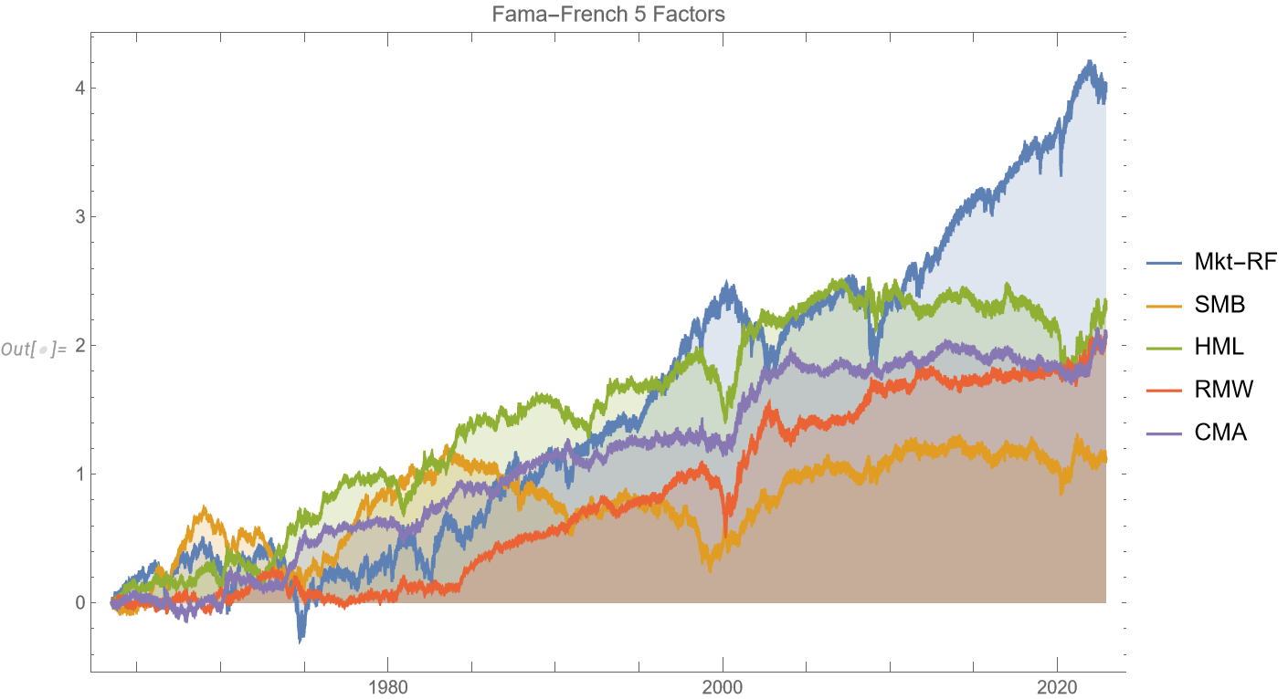
A follow-up extract from my forthcoming book, Equity Analytics
Applying-Factor-Models-in-Pairs-TradingApplying Factor Models in Pairs Trading

QUANTITATIVE RESEARCH AND TRADING
The latest theories, models and investment strategies in quantitative research and trading
A follow-up extract from my forthcoming book, Equity Analytics
Applying-Factor-Models-in-Pairs-Trading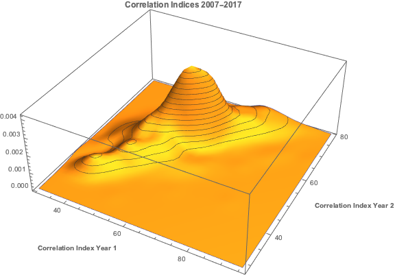
In a previous post I looked at ways of modeling the relationship between the CBOE VIX Index and the Year 1 and Year 2 CBOE Correlation Indices:
http://jonathankinlay.com/2017/08/modeling-volatility-correlation/
The question was put to me whether the VIX and correlation indices might be cointegrated.
Let’s begin by looking at the pattern of correlation between the three indices:
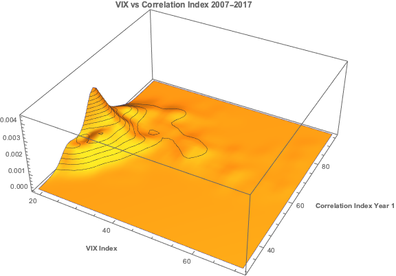
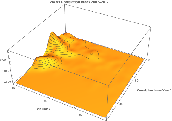
If you recall from my previous post, we were able to fit a linear regression model with the Year 1 and Year 2 Correlation Indices that accounts for around 50% in the variation in the VIX index. While the model certainly has its shortcomings, as explained in the post, it will serve the purpose of demonstrating that the three series are cointegrated. The standard Dickey-Fuller test rejects the null hypothesis of a unit root in the residuals of the linear model, confirming that the three series are cointegrated, order 1.


We can attempt to take the modeling a little further by fitting a VAR model. We begin by splitting the data into an in-sample period from Jan 2007 to Dec 2015 and an out-of-sample test period from Jan 2016 to Aug 2017. We then fit a vector autoregression model to the in-sample data:
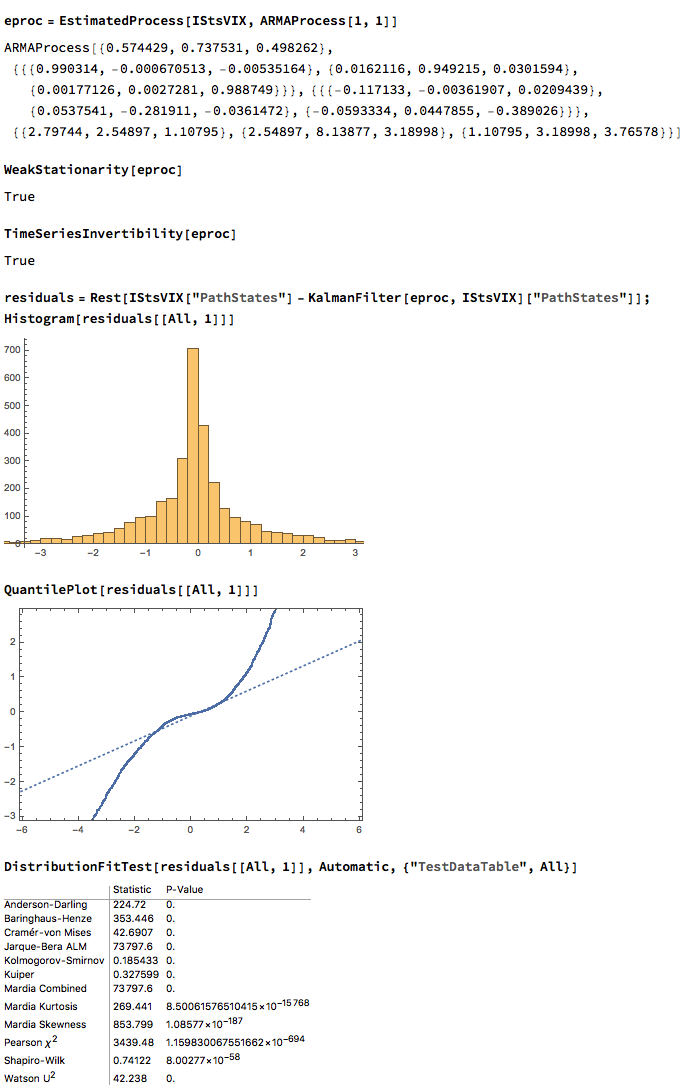
When we examine how the model performs on the out-of-sample data, we find that it fails to pick up on much of the variation in the series – the forecasts are fairly flat and provide quite poor predictions of the trends in the three series over the period from 2016-2017:
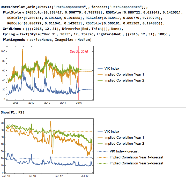
The VIX and Correlation Indices are not only highly correlated, but also cointegrated, in the sense that a linear combination of the series is stationary.
One can fit a weakly stationary VAR process model to the three series, but the fit is quite poor and forecasts from the model don’t appear to add much value. It is conceivable that a more comprehensive model involving longer lags would improve forecasting performance.
For those who prefer a little more rigor in their quantitative research, I can offer more a somewhat more substantive statistical argument in favor of the IBS indicator discussed in my previous post.
Specifically, we can show quite convincingly that the IBS process is stationary, a highly desirable property much sought-after in, for example, the construction of statistical arbitrage strategies. Of course, by construction, the IBS is constrained to lie between the values of 0 and 1, so non-stationarity in the mean is highly unlikely. But, conceivably, there could be some time dependency in the process or in its variance, for instance. Then there is the further question as to whether the IBS indicator is mean-reverting, which would indicate that the underlying price process likewise has a tendency to mean revert.
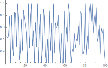
Let’s take the IBS series for Exxon-Mobil (XOM) as an example to work with. I have computed the series from the beginning of 1990, and the first 100 values are shown in the plot below.
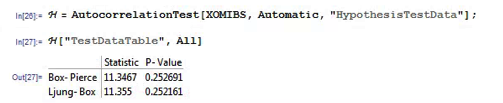
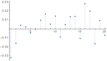
There appears to be little patterning in the process autocorrelations, and this is confirmed by formal statistical tests which fail to reject the null hypothesis that the first 20 autocorrelations are not, collectively, statistically significant.
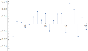
Next we test for the presence of a unit root in the IBS process (highly unlikely, given its construction) and indeed, unsurprisingly, the null hypothesis of a unit root is roundly rejected by the Dickey-Fuller and Phillips-Perron tests.

We next conduct a formal test to determine whether the IBS series follows a random walk.
The variance ratio test assesses the null hypothesis that a univariate time series y is a random walk. The null model is
y(t) = c + y(t–1) + e(t),
where c is a drift constant (assumed zero for the IBS series) and e(t) are uncorrelated innovations with zero mean.
IID is false, the alternative is that the e(t) are correlated.IID is true, the alternative is that the e(t) are either dependent or not identically distributed (for example, heteroscedastic).
We test whether the XOM IBS series is a random walk using various step sizes and perform the test with and without the assumption that the innovations are independent and identically distributed.
Switching to Matlab, we proceed as follows:
q = [2 4 8 2 4 8];
flag = logical([1 1 1 0 0 0]);
[h,pValue,stat,cValue,ratio] = vratiotest(XOMIBS,’period’,q,’IID’,flag)
Here h is a vector of Boolean decisions for the tests, with length equal to the number of tests. Values of h equal to 1 indicate rejection of the random-walk null in favor of the alternative. Values of h equal to 0 indicate a failure to reject the random-walk null.
The variable ratio is a vector of variance ratios, with length equal to the number of tests. Each ratio is the ratio of:
For a random walk, these ratios are asymptotically equal to one. For a mean-reverting series, the ratios are less than one. For a mean-averting series, the ratios are greater than one.
For the XOM IBS process we obtain the following results:
h = 1 1 1 1 1 1
pValue = 1.0e-51 * [0.0000 0.0000 0.0000 0.0000 0.0000 0.1027]
stat = -27.9267 -21.7401 -15.9374 -25.1412 -20.2611 -15.2808
cValue = 1.9600 1.9600 1.9600 1.9600 1.9600 1.9600
ratio = 0.4787 0.2405 0.1191 0.4787 0.2405 0.1191
The random walk hypothesis is convincingly rejected for both IID and non-IID error terms. The very low ratio values indicate that the IBS process is strongly mean reverting.
While standard statistical tests fail to find evidence of any non-stationarity in the Internal Bar Strength signal for Exxon-Mobil, the hypothesis that the series follows a random walk (with zero drift) is roundly rejected by variance ratio tests. These tests also confirm that the IBS series is strongly mean reverting, as we previously discovered empirically.
This represents an ideal scenario for trading purposes: a signal with the highly desirable properties that is both stationary and mean reverting. In the case of Exxon-Mobil, there appears to be clear evidence from both statistical tests and empirical trading strategies using the Internal Bar Strength indicator that the tendency of the price series to mean-revert is economically as well as statistically significant.

In this quantitative analysis I explore how, starting from the assumption of a stable, Gaussian distribution in a returns process, we evolve to a system that displays all the characteristics of empirical market data, notably time-dependent moments, high levels of kurtosis and fat tails. As it turns out, the only additional assumption one needs to make is that the market is periodically disturbed by the random arrival of news.
NOTE: if you are unable to see the Mathematica models below, you can download the free Wolfram CDF player and you may also need this plug-in.
You can also download the complete Mathematica CDF file here.
A stationary process is one that evolves over time, but whose probability distribution does not vary with time. As the word implies, such a process is stable. More formally, the moments of the distribution are independent of time.
Let’s assume we are dealing with such a process that have constant mean μ and constant volatility (standard deviation) σ.
Φ=NormalDistribution[μ,σ]
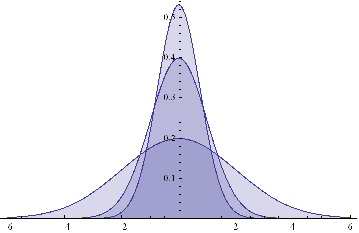
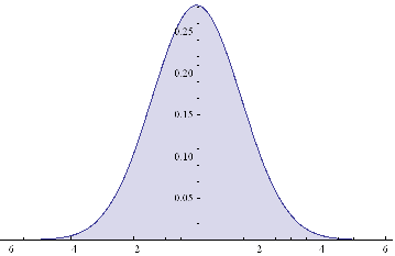
Here are some examples of Normal probability distributions, with constant mean μ = 0 and standard deviation σ ranging from 0.75 to 2
Plot[Evaluate@Table[PDF[Φ,x],{σ,{.75,1,2}}]/.μ→0,{x,-6,6},Filling→Axis]
The moments of Φ are given by:
Through[{Mean, StandardDeviation, Skewness, Kurtosis}[Φ]]
{μ, σ, 0, 3}
They, too, are time – independent.
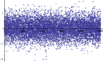
We can simulate some observations from such a process, with, say, mean μ = 0 and standard deviation σ = 1:
ListPlot[sampleData=RandomVariate[Φ /.{μ→0, σ→1},10^4]]
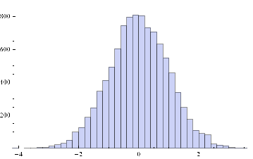
Histogram[sampleData]
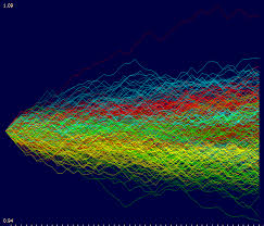
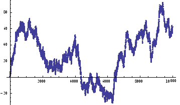
If we assume for the moment that such a process is an adequate description of an asset returns process, we can simulate the evolution of a price process as follows :
ListPlot[prices=Accumulate[sampleData]]
Lets take a look at a real price series, comprising 1 – minute bar data in the June ‘ 14 E – Mini futures contract.
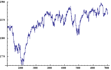
As with our simulated price process, it is clear that the real price process for Emini futures is also non – stationary.
What about the returns process?
ListPlot[returnsES]
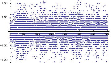
Notice the banding effect in returns, which results from having a fixed, minimum price move of $12 .50, rather than a continuous scale.
Histogram[returnsES]
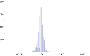
Through[{Min,Max,Mean,Median,StandardDeviation,Skewness,Kurtosis}[returnsES]]
{-0.00867214, 0.0112353, 2.75501×10⁻⁶, 0., 0.000780895, 0.35467, 26.2376}
The empirical returns distribution doesn’ t appear to be Gaussian – the distribution is much more peaked than a standard Normal distribution with the same mean and standard deviation. And the higher moments don’t fit the Normal model either – the empirical distribution has positive skew and a kurtosis that is almost 9x greater than a Gaussian distribution. The latter signifies what is often referred to as “fat tails”: the distribution has much greater weight in the tails than a standard Normal distribution, indicating a much greater likelihood of an extreme value than a Normal distribution would predict.
Non – stationarity arises when one or more of the moments of a distribution vary over time. Let’s take a look at how that can arise, and its effects.Suppose we have a Gaussian returns process for which the mean, or drift, or trend, fluctuates over time.
Let’s consider a simple example where the process drift is μ1 and volatility σ1 for most of the time and then for some proportion of time k, we get addition drift μ2 and volatility σ2. In other words we have:
Φ1=NormalDistribution[μ1,σ1]
Through[{Mean,StandardDeviation,Skewness,Kurtosis}[Φ1]]
{μ1, σ1, 0, 3}
Φ2=NormalDistribution[μ2,σ2]
Through[{Mean,StandardDeviation,Skewness,Kurtosis}[Φ2]]
{μ2, σ2, 0, 3}
This simple model fits a scenario in which we suppose that the returns process spends most of its time in State 1, in which is Normally distributed with drift is μ1 and volatility σ1, and suffers from the occasional “shock” which propels the systems into a second State 2, in which its distribution is a combination of its original distribution and a new Gaussian distribution with different mean and volatility.
Let’ s suppose that we sample the combined process y = Φ1 + k Φ2. What distribution would it have? We can represent this is follows :
y=TransformedDistribution[(x1+k x2),{x1~Φ1,x2~Φ2}]
Through[{Mean,StandardDeviation,Skewness,Kurtosis}[y]]
![]()
Plot[PDF[y,x]/.{μ1→0,μ2→0,σ1 →1,σ2 →2, k→0.5},{x,-6,6},Filling→Axis]
The result is just another Normal distribution. Depending on the incidence k, y will follow a Gaussian distribution whose mean and variance depend on the mean and variance of the two Normal distributions being mixed. The resulting distribution in State 2 may have higher or lower drift and volatility, but it is still Gaussian, with constant kurtosis of 3.
In other words, the system y will be non-stationary, because the first and second moments change over time, depending on what state it is in. But the form of the distribution is unchanged – it is still Gaussian. There are no fat-tails.
In the above example the system moved between states in a known, predictable way. The “shocks” to the system were not really shocks, but transitions. But that’s not how financial markets behave: markets move from one state to another in an unpredictable way, with the arrival of news.
We can simulate this situation as follows. Using the former model as a starting point, lets now relax the assumption that the incidence of the second state, k, is a constant. Instead, let’ s assume that k is itself a random variable. In other words we are going to now assume that our system changes state in a random way. How does this alter the distribution?
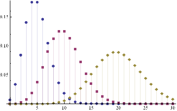
An appropriate model for λ might be a Poisson process, which is often used as a model for unpredictable, discrete events, ranging from bus arrivals to earthquakes. PDFs of Poisson distributions with means λ=5, 10 and 20 are shown in the chart below. These represent probability distributions for processes that have mean arrivals of 5, 10 or 20 events.
DiscretePlot[Evaluate@Table[PDF[PoissonDistribution[λ],k],{λ,{5,10,20}}],{k,0,30},PlotRange→All,PlotMarkers→Automatic]
Our new model now looks like this :
y=TransformedDistribution[{x1+k*x2},{x1⎡Φ1,x2⎡Φ2,k⎡PoissonDistribution[λ]}]
The first two moments of the distribution are as follows :
Through[{Mean,StandardDeviation}[y]]
![]()
As before, the mean and standard deviation of the distribution are going to vary, depending on the state of the system, and the mean arrival rate of shocks, . But what about kurtosis? Is it still constant?
Kurtosis[y]
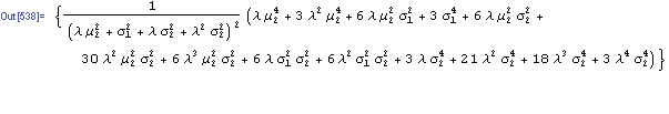
Emphatically not! The fourth moment of the distribution is now dependent on the drift in the second state, the volatilities of both states and the mean arrival rate of shocks, λ.
Let’ s look at a specific example. Assume that in State 1 the process has volatility of 7.5 %, with zero drift, and that the shock distribution also has zero drift with volatility of 65 %. If the mean incidence rate of shocks λ = 10 %, the distribution kurtosis is close to that seen in the empirical distribution for the E-Mini.
Kurtosis[y] /.{σ1→0.075,μ2→0,σ2→0.65,λ→0.1}
{35.3551}
More generally :
ListLinePlot[Flatten[Kurtosis[y]/.Table[{σ1→0.075,μ2→0,σ2→0.65,λ→i/20},{i,1,20}]],PlotLabel→Style[“Kurtosis vs Mean Shock Arrival Rate”, FontSize→18],AxesLabel->{“Incidence Rate (%)”, “Kurtosis”},Filling→Axis, ImageSize→Large]
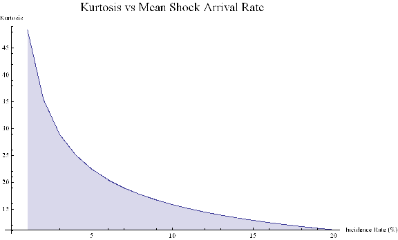
Thus we can see how, even if the underlying returns distribution is Gaussian in form, the random arrival of news “shocks” to the system can induce non – stationarity in overall drift and volatility. It can also result in fat tails. More specifically, if the arrival of news is stochastic in nature, rather than deterministic, the process may exhibit far higher levels of kurtosis than in its original Gaussian state, in which the fourth moment was a constant level of 3.
Nobel – prize winning economist Robert Merton extended this basic concept to the realm of stochastic calculus.
In Merton’s jump diffusion model, the stock price follows the random process
∂St / St =μdt + σdWt+(J-1)dNt
The first two terms are familiar from the Black–Scholes model : drift rate μ, volatility σ, and random walk Wt (Wiener process).The last term represents the jumps :J is the jump size as a multiple of stock price, while Nt is the number of jump events that have occurred up to time t.is assumed to follow the Poisson process.
PDF[PoissonDistribution[λt]]
where λ is the average frequency with which jumps occur.
The jump size J follows a log – normal distribution
PDF[LogNormalDistribution[m, ν], s]
where m is the average jump size and v is the volatility of the jump size.
In the jump diffusion model, the stock price St follows the random process dSt/St=μ dt+σ dWt+(J-1) dN(t), which comprises, in order, drift, diffusive, and jump components. The jumps occur according to a Poisson distribution and their size follows a log-normal distribution. The model is characterized by the diffusive volatility σ, the average jump size J (expressed as a fraction of St), the frequency of jumps λ, and the volatility of jump size ν.
The “implied volatility” corresponding to an option price is the value of the volatility parameter for which the Black-Scholes model gives the same price. A well-known phenomenon in market option prices is the “volatility smile”, in which the implied volatility increases for strike values away from the spot price. The jump diffusion model is a generalization of Black–Scholes in which the stock price has randomly occurring jumps in addition to the random walk behavior. One of the interesting properties of this model is that it displays the volatility smile effect. In this Demonstration, we explore the Black–Scholes implied volatility of option prices (equal for both put and call options) in the jump diffusion model. The implied volatility is modeled as a function of the ratio of option strike price to spot price.