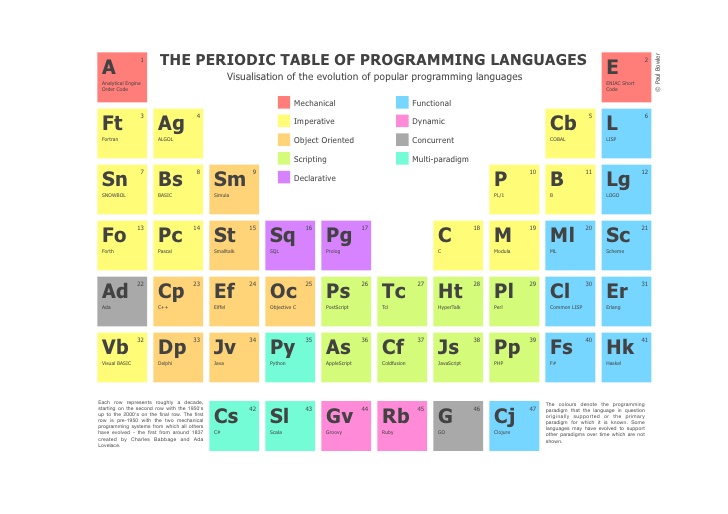
October 2, 2018 - QUANTITATIVE RESEARCH AND TRADING

Towards the end of last year I wrote a post (see here) about the advent of modern programming languages, including the JIT compiled Julia and visual programming language ADL from Trading Technologies. My conclusion (based on a not very scientific sample) was that we appear to be at the tipping point, where the speed of newer, high level languages languages is approaching that of the fastest compiled languages like C/C++.

Now comes a formal academic study of the topic in A Comparison of Programming Languages in Economics, Aruoba and Fernandez-Villaverde, 2014. Using the neoclassical growth model, the authors conduct a benchmark test in C++11, Fortran 2008, Java, Julia, Python, Matlab, Mathematica, and R, implementing the same algorithm, value function
iteration with grid search, in each of the languages. They report the execution times of the codes in a Mac and in a Windows computer and briefly comment on the strengths and weaknesses of each language.

The conclusions from the study mirror my own thoughts on the subject very closely. The authors find that:

C++ and Fortran are still considerably faster than any other alternative, although one needs to be careful with the choice of compiler.
C++ compilers have advanced enough that, contrary to the situation in the 1990s and some folk wisdom, C++ code runs slightly faster (5-7 percent) than Fortran code.
Julia delivers outstanding performance. Execution speed is only between 2.64 and 2.70 times slower than the execution speed of the best C++ compiler.
Baseline Python was slow. Using the Pypy implementation, it runs around 44 times slower than in C++. Using the default CPython interpreter, the code runs between 155 and 269 times slower than in C++.
Matlab is between 9 to 11 times slower than the best C++ executable.
R runs between 475 to 491 times slower than C++. If the code is compiled, the code is between 243 to 282 times slower.
Hybrid programming and special approaches can deliver considerable speed ups. For example, when combined with Mex files, Matlab is only 1.24 to 1.64 times slower than C++ and when combined with Rcpp, R is between 3.66 and 5.41 times slower. Similar numbers hold for Numba (a just-in-time compiler for Python that uses decorators) and Cython (a static compiler for writing C extensions for Python) in the Python ecosystem.
Mathematica is only about three times slower than C++, but only after a considerable rewriting of the code to take advantage of the peculiarities of the language. The baseline version of the algorithm in Mathematica is considerably slower.

C++ still represents the benchmark for speed, but not by much. It is barely faster than the old stalwart, Fortran, and only 1.5 – 3 times faster than up-and-coming rivals amongst the higher level languages (especially when you allow for hybrid programming to speed up the slowest algorithms).

So, as regards developing financial models and trading systems, my questions are (as before):

Why would anyone prefer Python, given that there is a much faster, free alternative in Julia, which is just as easy a language to program in?
What justification is there for preferring R to Matlab, other than cost?
Why does anyone bother with Java? If speed is the critical issue, there are faster alternatives. If you like the relative simplicity of the syntax, Julia is cleaner, simpler and just as fast in execution.

When you reach a point where a high level language like Matlab is only around 1.5x – 2x slower than C++, you really have to question whether the latter is an appropriate choice. Yes, of course, in mission-critical applications where you need access to the hardware layer for speed purposes, C++ is the way to go. But for so many applications, that just isn’t the case.

What matters, far, far more, are the months of costly and laborious programming effort that is often required to reproduce basic functionality that is already embedded in higher level languages like Matlab or Mathematica. Not only that, but the end result of a C++ /Java development effort is likely to be notoriously inflexible by comparison. That’s a huge drawback. Rarely, if ever, does a piece of research translate flawlessly into production – it requires one to iterate towards a final solution, often making significant changes to the design of the system in the light of practical experience.

If I had to guess, based on my experience, I would say that 80% or more of development tasks in quantitative research and trading would produce a superior result if preference was given to using a higher level language for the initial development. When the system is sufficiently stable to put into production, you simply create a hybrid application by recoding any mission-critical components for which speed is an issue in C++.

Finally, where does that leave my beloved Mathematica? To be fair, while you don’t have the joys of strong typing to contend with, Mathematica’s syntax is just as demanding and uncompromising as C++ – a missed comma or incorrectly placed bracket is just as critical. But, the point is, while in C++ the syntactical rigor is just annoying, in Mathematica it’s worth putting up with because the productivity is so much greater. A competent programmer can produce, in a single line of Mathematica code, a program that would require hundreds, if not thousands of lines of C++ code to accomplish. Sure, he might get the syntax wrong at first: but it’s only a single line of code and the interactive gui interface makes debugging very simple.

That said, while Mathematica can be very tedious to use for procedural programming, it excels in three areas:

1. Symbolic programming. Anything involving mathematical symbols and equations – Mathematica is #1

2. User interface. In Mathematica, it is trivial to build a sophisticated, dynamic gui in no time at all, again, often in 1-2 lines of code

3. Functional programming. Anything that can be thought of as a function, Mathematica handles extremely well. We are not talking about finding a square root here: I mean extremely complex functions that, again, might take hundreds of lines of code in another language.

It is also worth pointing out that Mathematica comes supplied with functionality that Matlab provides only through numerous, costly add-on packages.

CONCLUSION
Before I allow a development team to start mindlessly coding up a system in Java or C++, I want to hear their reasons why they aren’t going to do it 10x faster in another, higher level language. “We always use C++/Java for production” is not a reason. Specifically, which parts of the system require the additional 1.5x speed-up, and why can’t they be coded as dlls (Matlab mex functions)?

Finally, on a cost-benefit basis, ask yourself how much you might benefit if the months and tens (or hundreds) of thousands of dollars wasted on developing in C++ were instead spent on researching and developing new trading ideas.

Quant Strategies – Performance Summary Sept. 2018

The end of Q3 seems like an appropriate time for an across-the-piste review of how systematic strategies are performing in 2018. I’m using the dozen or more strategies running on the Systematic Algotrading Platform as the basis for the performance review, although results will obviously vary according to the specifics of the strategy. All of the strategies are traded live and performance results are net of subscription fees, as well as slippage and brokerage commissions.

Volatility Strategies

Those waiting for the hammer to fall on option premium collecting strategies will have been disappointed with the way things have turned out so far in 2018. Yes, February saw a long-awaited and rather spectacular explosion in volatility which completely destroyed several major volatility funds, including the VelocityShares Daily Inverse VIX Short-Term ETN (XIV) as well as Chicago-based hedged fund LJM Partners (“our goal is to preserve as much capital as possible”), that got caught on the wrong side of the popular VIX carry trade. But the lack of follow-through has given many volatility strategies time to recover. Indeed, some are positively thriving now that elevated levels in the VIX have finally lifted option premiums from the bargain basement levels they were languishing at prior to February’s carnage. The Option Trader strategy is a stand-out in this regard: not only did the strategy produce exceptional returns during the February melt-down (+27.1%), the strategy has continued to outperform as the year has progressed and YTD returns now total a little over 69%. Nor is the strategy itself exceptionally volatility: the Sharpe ratio has remained consistently above 2 over several years.

Hedged Volatility Trading

Investors’ chief concern with strategies that rely on collecting option premiums is that eventually they may blow up. For those looking for a more nuanced approach to managing tail risk the Hedged Volatility strategy may be the way to go. Like many strategies in the volatility space the strategy looks to generate alpha by trading VIX ETF products; but unlike the great majority of competitor offerings, this strategy also uses ETF options to hedge tail risk exposure. While hedging costs certainly acts as a performance drag, the results over the last few years have been compelling: a CAGR of 52% with a Sharpe Ratio close to 2.

F/X Strategies

One of the common concerns for investors is how to diversify their investment portfolios, especially since the great majority of assets (and strategies) tend to exhibit significant positive correlation to equity indices these days. One of the characteristics we most appreciate about F/X strategies in general and the F/X Momentum strategy in particular is that its correlation to the equity markets over the last several years has been negligible. Other attractive features of the strategy include the exceptionally high win rate – over 90% – and the profit factor of 5.4, which makes life very comfortable for investors. After a moderate performance in 2017, the strategy has rebounded this year and is up 56% YTD, with a CAGR of 64.5% and Sharpe Ratio of 1.89.

Equity Long/Short

Thanks to the Fed’s accommodative stance, equity markets have been generally benign over the last decade to the benefit of most equity long-only and long-short strategies, including our equity long/short Turtle Trader strategy , which is up 31% YTD. This follows a spectacular 2017 (+66%) , and is in line with the 5-year CAGR of 39%. Notably, the correlation with the benchmark S&P500 Index is relatively low (0.16), while the Sharpe Ratio is a respectable 1.47.

Equity ETFs – Market Timing/Swing Trading

One alternative to the traditional equity long/short products is the Tech Momentum strategy. This is a swing trading strategy that exploits short term momentum signals to trade the ProShares UltraPro QQQ (TQQQ) and ProShares UltraPro Short QQQ (SQQQ) leveraged ETFs. The strategy is enjoying a banner year, up 57% YTD, with a four-year CAGR of 47.7% and Sharpe Ratio of 1.77. A standout feature of this equity strategy is its almost zero correlation with the S&P 500 Index. It is worth noting that this strategy also performed very well during the market decline in Feb, recording a gain of over 11% for the month.

Futures Strategies

It’s a little early to assess the performance of the various futures strategies in the Systematic Strategies portfolio, which were launched on the platform only a few months ago (despite being traded live for far longer). For what it is worth, both of the S&P 500 E-Mini strategies, the Daytrader and the Swing Trader, are now firmly in positive territory for 2018. Obviously we are keeping a watchful eye to see if the performance going forward remains in line with past results, but our experience of trading these strategies gives us cause for optimism.

Conclusion: Quant Strategies in 2018

There appear to be ample opportunities for investors in the quant sector across a wide range of asset classes. For investors with equity market exposure, we particularly like strategies with low market correlation that offer significant diversification benefits, such as the F/X Momentum and F/X Momentum strategies. For those investors seeking the highest risk adjusted return, option selling strategies like the Option Trader strategy are the best choice, while for more cautious investors concerned about tail risk the Hedged Volatility strategy offers the security of downside protection. Finally, there are several new strategies in equities and futures coming down the pike, several of which are already showing considerable promise. We will review the performance of these newer strategies at the end of the year.

Go here for more information about the Systematic Algotrading Platform.