January 2019 - QUANTITATIVE RESEARCH AND TRADING

January 29, 2019

Improving Trading System Performance Using a Meta-Strategy

What is a Meta-Strategy?

In my previous post on identifying drivers of strategy performance I mentioned the possibility of developing a meta-strategy.

A meta-strategy is a trading system that trades trading systems. The idea is to develop a strategy that will make sensible decisions about when to trade a specific system, in a way that yields superior performance compared to simply following the underlying trading system. Put another way, the simplest kind of meta-strategy is a long-only strategy that takes positions in some underlying trading system. At times, it will follow the underlying system exactly; at other times it is out of the market and ignore the trading system’s recommendations.

More generally, a meta-strategy can determine the size in which one, or several, systems should be traded at any point in time, including periods where the size can be zero (i.e. the system is not currently traded). Typically, a meta-strategy is long-only: in theory there is nothing to stop you developing a meta-strategy that shorts your underlying strategy from time to time, but that is a little counter-intuitive to say the least!

A meta-strategy is something that could be very useful for a fund-of-funds, as a way of deciding how to allocate capital amongst managers.

Caissa Capital operated a meta-strategy in its option arbitrage hedge fund back in the early 2000’s. The meta-strategy (we called it a “model management system”) selected from a half dozen different volatility models to be used for option pricing, depending their performance, as measured by around 30 different criteria. The criteria included both statistical metrics, such as the mean absolute percentage error in the forward volatility forecasts, as well as trading performance criteria such as the moving average of the trade PNL. The model management system probably added 100 – 200 basis points per annum to the performance the underlying strategy, so it was a valuable add-on.

Illustration of a Meta-Strategy in US Bond Futures

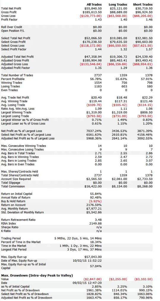
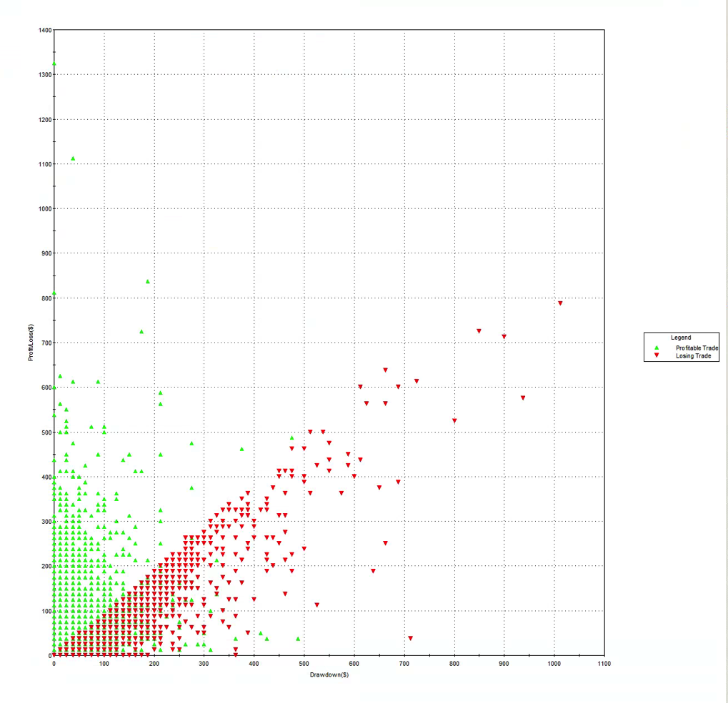
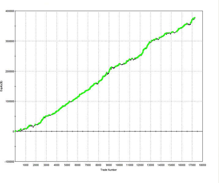
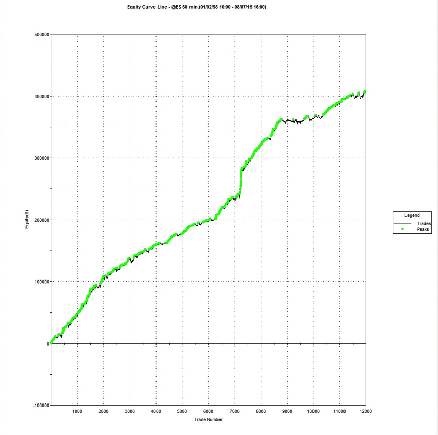
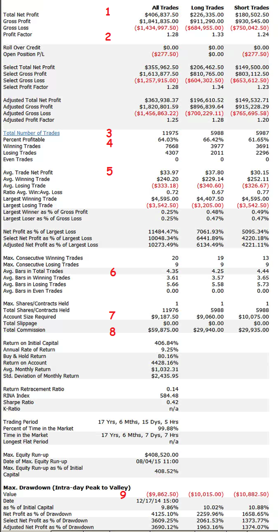
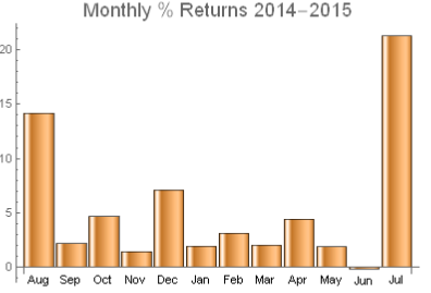
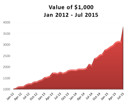
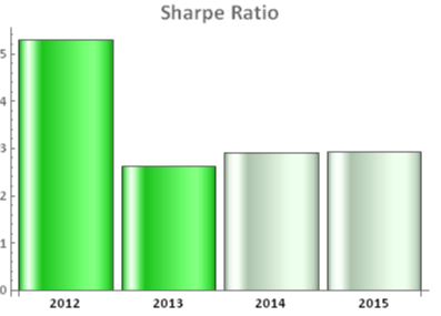
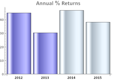
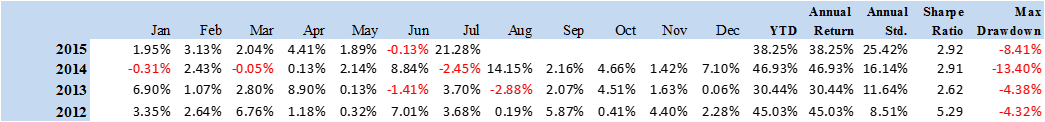
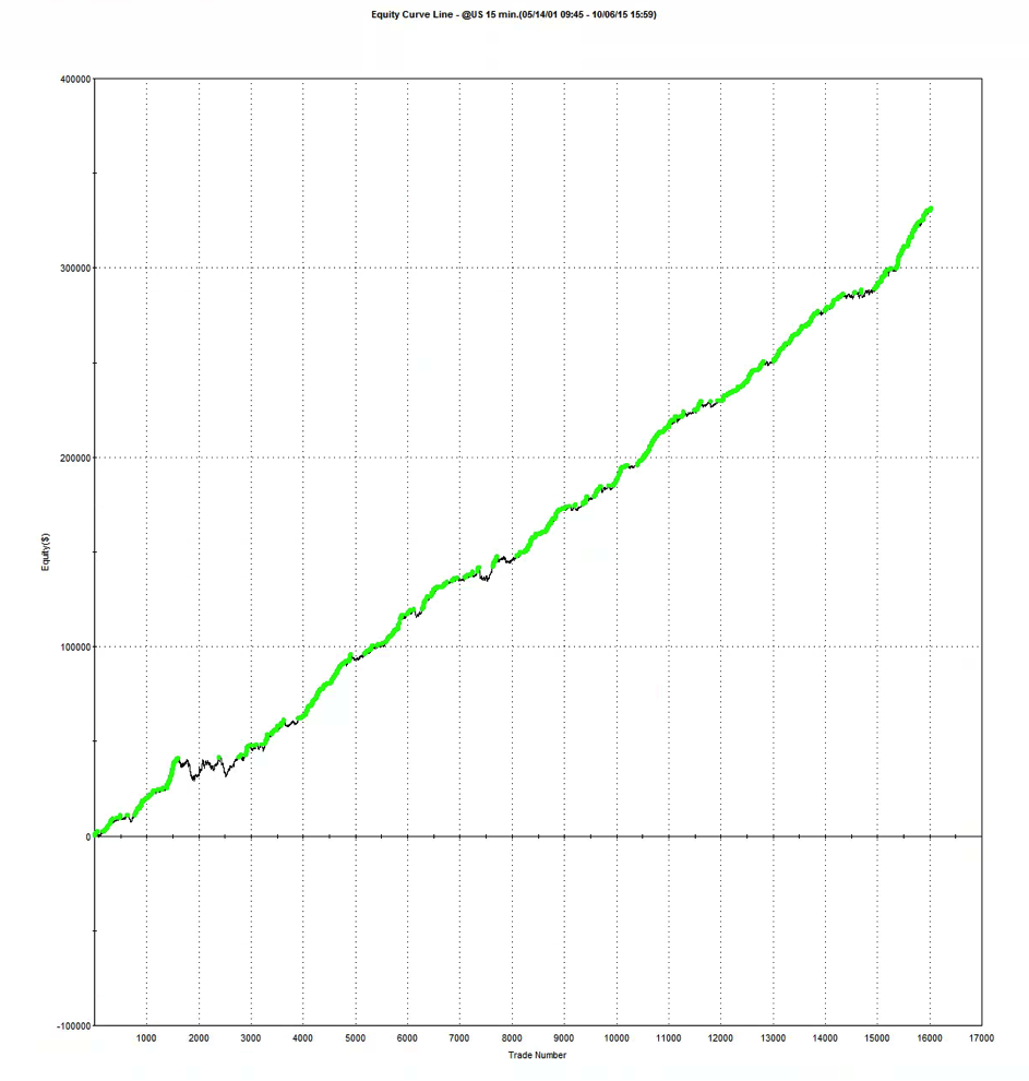
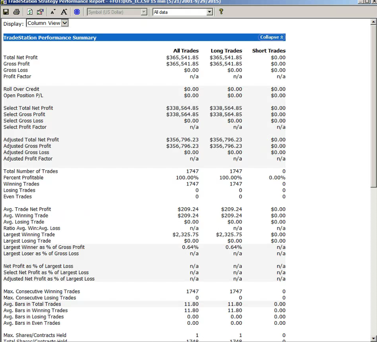
To illustrate the concept we will use an underlying system that trades US Bond futures at 15-minute bar intervals. The performance of the system is summarized in the chart and table below.

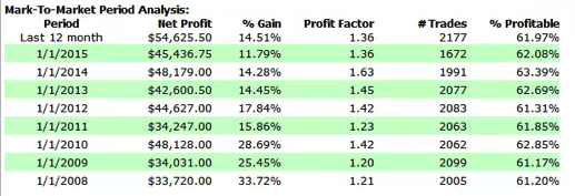
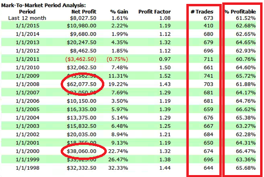
Strategy performance has been very consistent over the last seven years, in terms of the annual returns, number of trades and % win rate. Can it be improved further?

To assess this possibility we create a new data series comprising the points of the equity curve illustrated above. More specifically, we form a series comprising the open, high, low and close values of the strategy equity, for each trade. We will proceed to treat this as a new data series and apply a range of different modeling techniques to see if we can develop a trading strategy, in exactly the same way as we would if the underlying was a price series for a stock.

It is important to note here that, for the meta-strategy at least, we are working in trade-time, not calendar time. The x-axis will measure the trade number of the underlying strategy, rather than the date of entry (or exit) of the underlying trade. Thus equally spaced points on the x-axis represent different lengths of calendar time, depending on the duration of each trade.

It is necessary to work in trade time rather than calendar time because, unlike a stock, it isn’t possible to trade the underlying strategy whenever we want to – we can only enter or exit the strategy at points in time when it is about to take a trade, by accepting that trade or passing on it (we ignore the other possibility which is sizing the underlying trade, for now).

Another question is what kinds of trading ideas do we want to consider for the meta-strategy? In principle one could incorporate almost any trading concept, including the usual range of technical indictors such as RSI, or Bollinger bands. One can go further an use machine learning techniques, including Neural Networks, Random Forest, or SVM.

In practice, one tends to gravitate towards the simpler kinds of trading algorithm, such as moving averages (or MA crossover techniques), although there is nothing to say that more complex trading rules should not be considered. The development process follows a familiar path: you create a hypothesis, for example, that the equity curve of the underlying bond futures strategy tends to be mean-reverting, and then proceed to test it using various signals – perhaps a moving average, in this case. If the signal results in a potential improvement in the performance of the default meta-strategy (which is to take every trade in the underlying system system), one includes it in the library of signals that may ultimately be combined to create the finished meta-strategy.

As with any strategy development you should follows the usual procedure of separating the trade data to create a set used for in-sample modeling and out-of-sample performance testing.

Following this general procedure I arrived at the following meta-strategy for the bond futures trading system.

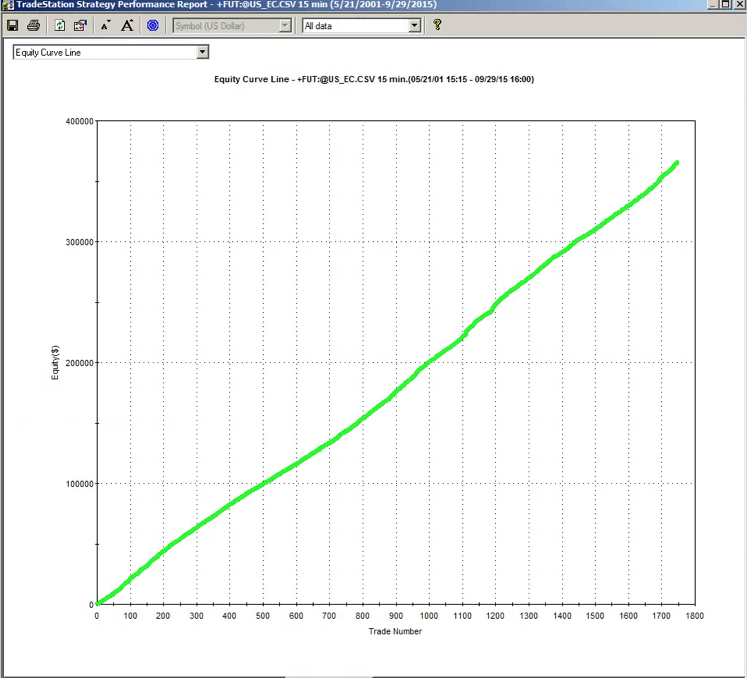
The modeling procedure for the meta-strategy has succeeded in eliminating all of the losing trades in the underlying bond futures system, during both in-sample and out-of-sample periods (comprising the most recent 20% of trades).

In general, it is unlikely that one can hope to improve the performance of the underlying strategy quite as much as this, of course. But it may well be possible to eliminate a sufficient proportion of losing trades to reduce the equity curve drawdown and/or increase the overall Sharpe ratio by a significant amount.

A Challenge / Opportunity

If you like the meta-strategy concept, but are unsure how to proceed, I may be able to help.

Send me the data for your existing strategy (see details below) and I will attempt to model a meta-strategy and send you the results. We can together evaluate to what extent I have been successful in improving the performance of the underlying strategy.

Here are the details of what you need to do:

1. You must have an existing, profitable strategy, with sufficient performance history (either real, simulated, or a mixture of the two). I don’t need to know the details of the underlying strategy, or even what it is trading, although it would be helpful to have that information.

2. You must send the complete history of the equity curve of the underlying strategy, in Excel format, with column headings Date, Open, High, Low, Close. Each row represents consecutive trades of the underlying system and the O/H/L/C refers to the value of the equity curve for each trade.

3. The history must comprise at least 500 trades as an absolute minimum and preferably 1000 trades, or more.

4. At this stage I can only consider a single underlying strategy (i.e. a single equity curve)

5. You should not include any software or algorithms of any kind. Nothing proprietary, in other words.

6. I will give preference to strategies that have a (partial) live track record.

As my time is very limited these days I will not be able to deal with any submissions that fail to meet these specifications, or to enter into general discussions about the trading strategy with you.

You can reach me at jkinlay@systematic-strategies.com

January 22, 2019

Identifying Drivers of Trading Strategy Performance

Building a winning strategy, like the one in the e-Mini S&P500 futures described here is only half the challenge: it remains for the strategy architect to gain an understanding of the sources of strategy alpha, and risk. This means identifying the factors that drive strategy performance and, ideally, building a model so that their relative importance can be evaluated. A more advanced step is the construction of a meta-model that will predict strategy performance and provided recommendations as to whether the strategy should be traded over the upcoming period.

Strategy Performance – Case Study

Let’s take a look at how this works in practice. Our case study makes use of the following daytrading strategy in e-Mini futures.

The overall performance of the strategy is quite good. Average monthly PNL over the period from April to Oct 2015 is almost $8,000 per contract, after fees, with a standard deviation of only $5,500. That equates to an annual Sharpe Ratio in the region of 5.0. On a decent execution platform the strategy should scale to around 10-15 contracts, with an annual PNL of around $1.0 to $1.5 million.

Looking into the performance more closely we find that the win rate (56%) and profit factor (1.43) are typical for a profitable strategy of medium frequency, trading around 20 times per session (in this case from 9:30AM to 4PM EST).

Another attractive feature of the strategy risk profile is the Max Adverse Execution, the drawdown experienced in individual trades (rather than the realized drawdown). In the chart below we see that the MAE increases steadily, without major outliers, to a maximum of only around $1,000 per contract.

One concern is that the average trade PL is rather small – $20, just over 1.5 ticks. Strategies that enter and exit with limit orders and have small average trade are generally highly dependent on the fill rate – i.e. the proportion of limit orders that are filled. If the fill rate is too low, the strategy will be left with too many missed trades on entry or exit, or both. This is likely to damage strategy performance, perhaps to a significant degree – see, for example my post on High Frequency Trading Strategies.

The fill rate is dependent on the number of limit orders posted at the extreme high or low of the bar, known as the extreme hit rate. In this case the strategy has been designed specifically to operate at an extreme hit rate of only around 10%, which means that, on average, only around one trade in ten occurs at the high or low of the bar. Consequently, the strategy is not highly fill-rate dependent and should execute satisfactorily even on a retail platform like Tradestation or Interactive Brokers.

Drivers of Strategy Performance

So far so good. But before we put the strategy into production, let’s try to understand some of the key factors that determine its performance. Hopefully that way we will be better placed to judge how profitable the strategy is likely to be as market conditions evolve.

In fact, we have already identified one potential key performance driver: the extreme hit rate (required fill rate) and determined that it is not a major concern in this case. However, in cases where the extreme hit rate rises to perhaps 20%, or more, the fill ratio is likely to become a major factor in determining the success of the strategy. It would be highly inadvisable to attempt implementation of such a strategy on a retail platform.

What other factors might affect strategy performance? The correct approach here is to apply the scientific method: develop some theories about the drivers of performance and see if we can find evidence to support them.

For this case study we might conjecture that, since the strategy enters and exits using limit orders, it should exhibit characteristics of a mean reversion strategy, which will tend to do better when the market moves sideways and rather worse in a strongly trending market.

Another hypothesis is that, in common with most day-trading and high frequency strategies, this strategy will produce better results during periods of higher market volatility. Empirically, HFT firms have always produced higher profits during volatile market conditions – 2008 was a banner year for many of them, for example. In broad terms, times when the market is whipsawing around create additional opportunities for strategies that seek to exploit temporary mis-pricings. We shall attempt to qualify this general understanding shortly. For now let’s try to gather some evidence that might support the hypotheses we have formulated.

I am going to take a very simple approach to this, using linear regression analysis. It’s possible to do much more sophisticated analysis using nonlinear methods, including machine learning techniques. In our regression model the dependent variable will be the daily strategy returns. In the first iteration, let’s use measures of market returns, trading volume and market volatility as the independent variables.

The first surprise is the size of the (adjusted) R Square – at 28%, this far exceeds the typical 5% to 10% level achieved in most such regression models, when applied to trading systems. In other words, this model does a very good job of account for a large proportion of the variation in strategy returns.

Note that the returns in the underlying S&P50o index play no part (the coefficient is not statistically significant). We might expect this: ours is is a trading strategy that is not specifically designed to be directional and has approximately equivalent performance characteristics on both the long and short side, as you can see from the performance report.

Now for the next surprise: the sign of the volatility coefficient. Our ex-ante hypothesis is that the strategy would benefit from higher levels of market volatility. In fact, the reverse appears to be true (due to the negative coefficient). How can this be? On further reflection, the reason why most HFT strategies tend to benefit from higher market volatility is that they are momentum strategies. A momentum strategy typically enters and exits using market orders and hence requires a major market move to overcome the drag of the bid-offer spread (assuming it calls the market direction correctly!). This strategy, by contrast, is a mean-reversion strategy, since entry/exits are effected using limit orders. The strategy wants the S&P500 index to revert to the mean – a large move that continues in the same direction is going to hurt, not help, this strategy.

Note, by contrast, that the coefficient for the volume factor is positive and statistically significant. Again this makes sense: as anyone who has traded the e-mini futures overnight can tell you, the market tends to make major moves when volume is light – simply because it is easier to push around. Conversely, during a heavy trading day there is likely to be significant opposition to a move in any direction. In other words, the market is more likely to trade sideways on days when trading volume is high, and this is beneficial for our strategy.

The final surprise and perhaps the greatest of all, is that the strategy alpha appears to be negative (and statistically significant)! How can this be? What the regression analysis appears to be telling us is that the strategy’s performance is largely determined by two underlying factors, volume and volatility.

Let’s dig into this a little more deeply with another regression, this time relating the current day’s strategy return to the prior day’s volume, volatility and market return.

In this regression model the strategy alpha is effectively zero and statistically insignificant, as is the case for lagged volume. The strategy returns relate inversely to the prior day’s market return, which again appears to make sense for a mean reversion strategy: our model anticipates that, in the mean, the market will reverse the prior day’s gain or loss. The coefficient for the lagged volatility factor is once again negative and statistically significant. This, too, makes sense: volatility tends to be highly autocorrelated, so if the strategy performance is dependent on market volatility during the current session, it is likely to show dependency on volatility in the prior day’s session also.

So, in summary, we can provisionally conclude that:

This strategy has no market directional predictive power: rather it is a pure, mean-reversal strategy that looks to make money by betting on a reversal in the prior session’s market direction. It will do better during periods when trading volume is high, and when market volatility is low.

Conclusion

Now that we have some understanding of where the strategy performance comes from, where do we go from here? The next steps might include some, or all, of the following:

(i) A more sophisticated econometric model bringing in additional lags of the explanatory variables and allowing for interaction effects between them.

(ii) Introducing additional exogenous variables that may have predictive power. Depending on the nature of the strategy, likely candidates might include related equity indices and futures contracts.

(iii) Constructing a predictive model and meta-strategy that would enable us assess the likely future performance of the strategy, and which could then be used to determine position size. Machine learning techniques can often be helpful in this content.

I will give an example of the latter approach in my next post.

January 15, 2019

Signal Processing and Sample Frequency

The Importance of Sample Frequency

Too often we apply a default time horizon for our trading, whether it below (daily, weekly) or higher (hourly, 5 minute) frequency. Sometimes the choice is dictated by practical considerations, such as a desire to avoid overnight risk, or the (lack of0 availability of low-latency execution platform.

But there is an alternative approach to the trade frequency decision that often yields superior results in terms of trading performance. The methodology derives from signal processing and the idea essentially is to use Fourier transforms to help identify the cyclical behavior of the strategy alpha and hence determine the best time-frames for sampling and trading. I wrote about this is a previous blog post, in which I described how to use principal components analysis to investigate the factors driving the returns in various pairs trading strategies. Here I want to take a simpler approach, in which we use Fourier analysis to select suitable sample frequencies. The idea is simply to select sample frequencies where the signal strength appears strongest, in the hope that it will lead to superior performance characteristics in what strategy we are trying to develop.

Signal Decomposition for S&P500 eMini Futures

Let’s take as an example the S&P 500 emini futures contract. The chart below shows the continuous ES futures contract plotted at 1-minute intervals from 1998. At the bottom of the chart I have represented the signal analysis as a bar chart (in blue), with each bar representing the amplitude at each frequency. The white dots on the chart identify frequencies that are spaced 10 minutes apart. It is immediately evident that local maxima in the spectrum occur around 40 mins, 60 mins and 120 mins. So a starting point for our strategy research might be to look at emini data sampled at these frequencies. Incidentally, it is worth pointing out that I have restricted the session times to 7AM – 4PM EST, which is where the bulk of the daily volume and liquidity tend to occur. You may get different results if you include data from the Globex session.

This is all very intuitive and unsurprising: the clearest signals occur at frequencies that most traders typically tend to trade, using hourly data, for example. Any strategy developer is already quite likely to consider these and other common frequencies as part of their regular research process. There are many instances of successful trading strategies built on emini data sampled at 60 minute intervals.

Signal Decomposition for US Bond Futures

Let’s look at a rather more interesting example: US (30 year) Bond futures. Unlike the emini contract, the spectral analysis of the US futures contract indicates that the strongest signal by far occurs at a frequency of around 47 minutes. This is decidedly an unintuitive outcome – I can’t think of any reason why such a strong signal should appear at this cycle length, but, statistically it does.

Does it work? Readers can judge for themselves: below is an example of an equity curve for a strategy on US futures sampled at 47 minute frequency over the period from 2002. The strategy has performed very consistently, producing around $25,000 per contract per year, after commissions and slippage.

Conclusion

While I have had similar success with products as diverse as Corn and VIX futures, the frequency domain approach is by no means a panacea: there are plenty of examples where I have been unable to construct profitable strategies for data sampled at the frequencies with very strong signals. Conversely, I have developed successful strategies using data at frequencies that hardly registered at all on the spectrum, but which I selected for other reasons. Nonetheless, spectral analysis (and signal processing in general) can be recommended as a useful tool in the arsenal of any quantitative analyst.

January 11, 2019January 11, 2019

A Universal Stock Screening Application

Happy New Year to my readers.

I recently pitched a consulting project that entailed building a stock screener that would apply both fundamental and technical criteria to identity a universe of candidate stocks across world-wide equity markets.

Here is how I approached the task:

StockScreener_1_4

January 8, 2019

Trading Strategy Design

In this post I want to share some thoughts on how to design great automated trading strategies – what to look for, and what to avoid.

For illustrative purposes I am going to use a strategy I designed for the ever-popular S&P500 e-mini futures contract.

The overall equity curve for the strategy is show below.

This is often the best place to start. What you want to see, of course, is a smooth, upward-sloping curve, without too many sizable drawdowns, and one in which the strategy continues to make new highs. This is especially important in the out-of-sample test period (Jan 2014- Jul 2015 in this case). You will notice a flat period around 2013, which we will need to explore later. Overall, however, this equity curve appears to fit the stereotypical pattern we hope to see when developing a new strategy.

Let’s move on look at the overall strategy performance numbers.

STRATEGY PERFORMANCE CHARACTERISTICS

(click to enlarge)

1. Net Profit
Clearly, the most important consideration. Over the 17 year test period the strategy has produced a net profit averaging around $23,000 per annum, per contract. As a rough guide, you would want to see a net profit per contract around 10x the maintenance margin, or higher.

2. Profit Factor
The gross profit divided by the gross loss. You want this to be as high as possible. Too low, as the strategy will be difficult to trade, because you will see sustained periods of substantial losses. I would suggest a minimum acceptable PF in the region of 1.25. Many strategy developers aim for a PF of 1.5, or higher.

3. Number of Trades
Generally, the more trades the better, at least from the point of view of building confidence in the robustness of strategy performance. A strategy may show a great P&L, but if it only trades once a month it is going to take many many years of performance data to ensure statistical significance. This strategy, on the other hand, is designed to trade 2-3 times a day. Given that, and the length of the test period, there is little doubt that the results are statistically significant.

Profit Factor and number of trades are opposing design criteria – increasing the # trades tends to reduce the PF. That consideration sets an upper bound on the # trades that can be accommodated, before the profit factor deteriorates to unacceptably low levels. Typically, 4-5 trades a day is about the maximum trading frequency one can expect to achieve.

4. Win Rate
Novice system designers tend to assume that you want this to be as high as possible, but that isn’t typically the case. It is perfectly feasible to design systems that have a 90% win rate, or higher, but which produce highly undesirable performance characteristics, such as frequent, large drawdowns. For a typical trading system the optimal range for the win rate is in the region of 40% to 66%. Below this range, it becomes difficult to tolerate the long sequences of losses that will result, without losing faith in the system.

5. Average Trade
This is the average net profit per trade. A typical range would be $10 to $100. Many designers will only consider strategies that have a higher average trade than this one, perhaps $50-$75, or more. The issue with systems that have a very small average trade is that the profits can quickly be eaten up by commissions. Even though, in this case, the results are net of commissions, one can see a significant deterioration in profits if the average trade is low and trade frequency is high, because of the risk of low fill rates (i.e. the % of limit orders that get filled). To assess this risk one looks at the number of fills assumed to take place at the high or low of the bar. If this exceeds 10% of the total # trades, one can expect to see some slippage in the P&L when the strategy is put into production.

6. Average Bars
The number of bars required to complete a trade, on average. There is no hard limit one can suggest here – it depends entirely on the size of the bars. Here we are working in 60 minute bars, so a typical trade is held for around 4.5 hours, on average. That’s a time-frame that I am comfortable with. Others may be prepared to hold positions for much longer – days, or even weeks.

Perhaps more important is the average length of losing trades. What you don’t want to see is the strategy taking far longer to exit losing trades than winning trades. Again, this is a matter of trader psychology – it is hard to sit there hour after hour, or day after day, in a losing position – the temptation to cut the position becomes hard to ignore. But, in doing that you are changing the strategy characteristics in a fundamental way, one that rarely produces a performance improvement.

What the strategy designer needs to do is to figure out in advance what the limits are of the investor’s tolerance for pain, in terms of maximum drawdown, average losing trade, etc, and design the strategy to meet those specifications, rather than trying to fix the strategy afterwards.

7. Required Account Size
It’s good to know exactly how large an account you need per contract, so you can figure out how to scale the strategy. In this case one could hope to scale the strategy up to a 10-lot in a $100,000 account. That may or may not fit the trader’s requirements and again, this needs to be considered at the outset. For example, for a trader looking to utilize, say, $1,000,000 of capital, it is doubtful whether this strategy would fit his requirements without considerable work on the implementations issues that arise when trying to trade in anything approaching a 100 contract clip rate.

8. Commission
Always check to ensure that the strategy designer has made reasonable assumptions about slippage and commission. Here we are assuming $5 per round turn. There is no slippage, because the strategy executes using limit orders.

9. Drawdown
Drawdowns are, of course, every investor’s bugbear. No-one likes drawdowns that are either large, or lengthy in relation to the annual profitability of the strategy, or the average trade duration. A $10,000 max drawdown on a strategy producing over $23,000 a year is actually quite decent – I have seen many e-mini strategies with drawdowns at 2x – 3x that level, or larger. Again, this is one of the key criteria that needs to be baked into the strategy design at the outset, rather than trying to fix later.

ANNUAL PROFITABILITY

Let’s now take a look at how the strategy performs year-by-year, and some of the considerations and concerns that often arise.

1. Performance During Downturns
One aspect I always pay attention to is how well the strategy performs during periods of high market stress, because I expect similar conditions to arise in the fairly near future, e.g. as the Fed begins to raise rates.

Here, as you can see, the strategy performed admirably during both the dot com bust of 1999/2000 and the financial crisis of 2008/09.

2. Consistency in the # Trades and % Win Rate
It is not uncommon with low frequency strategies to see periods of substantial variation in the # trades or win rate. Regardless how good the overall performance statistics are, this makes me uncomfortable. It could be, for instance, that the overall results are influenced by one or two exceptional years that are unlikely to be repeated. Significant variation in the trading or win rate raise questions about the robustness of the strategy, going forward. On the other hand, as here, it is a comfort to see the strategy maintaining a very steady trading rate and % win rate, year after year.

3. Down Years
Every strategy shows variation in year to year performance and one expects to see years in which the strategy performs less well, or even loses money. For me, it rather depends on when such losses arise, as much as the size of the loss. If a loss occurs in the out-of-sample period it raises serious questions about strategy robustness and, as a result, I am very unlikely to want to put such a strategy into production. If, as here, the period of poor performance occurs during the in-sample period I am less concerned – the strategy has other, favorable characteristics that make it attractive and I am willing to tolerate the risk of one modestly down-year in over 17 years of testing.

INTRA-TRADE DRAWDOWNS

Many trades that end up being profitable go through a period of being under-water. What matters here is how high those intra-trade losses may climb, before the trade is closed. To take an extreme example, would you be willing to risk $10,000 to make an average profit of only $10 per trade? How about $20,000? $50,000? Your entire equity?

The Maximum Average Excursion chart below shows the drawdowns on a trade by trade basis. Here we can see that, over the 17 year test period, no trade has suffered a drawdown of much more than $5,000. I am comfortable with that level. Others may prefer a lower limit, or be tolerant of a higher MAE.

Again, the point is that the problem of a too-high MAE is not something one can fix after the event. Sure, a stop loss will prevent any losses above a specified size. But a stop loss also has the unwanted effect of terminating trades that would have turned into money-makers. While psychologically comfortable, the effect of a stop loss is almost always negative in terms of strategy profitability and other performance characteristics, including drawdown, the very thing that investors are looking to control.

CONCLUSION
I have tried to give some general guidelines for factors that are of critical importance in strategy design. There are, of course, no absolutes: the “right” characteristics depend entirely on the risk preferences of the investor.

One point that strategy designers do need to take on board is the need to factor in all of the important design criteria at the outset, rather than trying (and usually failing) to repair the strategy shortcomings after the event.

January 1, 2019

My Big Fat Greek Vacation

LEARNING TO TRUST A TRADING SYSTEM

One of the most difficult decisions to make when running a systematic trading program is knowing when to override the system. During the early 2000’s when I was running the Caissa Capital fund, the models would regularly make predictions on volatility that I and our head Trader, Ron Henley, a former option trader from the AMEX, disagreed with. Most times, the system proved to have made the correct decision. My take-away from that experience was that, as human beings, even as traders, we are not very good at pricing risk.

My second take-away was that, by and large, you are better off trusting the system, rather than second-guessing its every decision. Of course, markets can change and systems break down; but the right approach to assessing this possibility is to use statistical control procedures to determine formally whether or not the system has broken down, rather than going through a routine period of under-performance (see: is your strategy still working?)

GREEK LESSONS

So when the Greek crisis blew up in June my first instinct was not to start looking immediately for the escape hatch. However, as time wore on I became increasingly concerned that the risk of a Grexit or default had not abated. Moreover, I realized that there was really nothing comparable in the data used in the development of the trading models that was in any way comparable to the scenario facing Greece, the EU and, by a process of contagion, US markets. Very reluctantly, therefore, I came to the decision that the smart way to play the crises was from the sidelines. So we made the decisions to go 100% to cash and waited for the crisis to subside.

A week went by. Then another. Of course, I had written to our investors explaining what we intended to do, and why, so there were no surprises. Nonetheless, I felt uncomfortable not making money for them. I did my best to console myself with the principal rule of money management: first, do not lose money. Of course we didn’t – but neither did we make much money, and ended June more or less flat.

COMEBACK

After the worst of the crisis was behind us, I was relieved to see that the models appeared almost as anxious as I was to make up for lost time. One of the features of the system is

that it makes aggressive use of leverage. Rather like an expert poker player, when it judges the odds to be in its favor, the system will increase its bet size considerably; at other times it will hunker down, play conservatively, or even exit altogether. Consequently, the turnover in the portfolio can be large at times. The cost of trading high volume can substantial, especially in some of the less liquid ETF products, where the bid/ask spread can amount to several cents. So we typically aim to execute passively, looking to buy on the bid and sell on the offer, using execution algos to split our orders up and randomize them. That also makes it tougher for HFT algos to pick us off as we move into and out of our positions.

So, in July, our Greek “vacation” at an end, the system came roaring back, all guns blazing. It quickly moved into some aggressive short volatility positions to take advantage of the elevated levels in the VIX, before reversing and gong long as the index collapsed to the bottom of the monthly range.

A DOUBLE-DIGIT MONTHLY RETURN: +21.28%

The results were rather spectacular: a return of +21.28% for the month, bringing the total return to 38.25% for 2015 YTD.

In the current low rate environment, this rate of return is extraordinary, but not entirely unprecedented: the strategy has produced double-digit monthly returns several times in the past, most recently in August last year, which saw a return of +14.1%. Prior, to that, the record had been +8.90% in April 2013.

Such outsized returns come at a price – they have the effect of increasing strategy volatility and hence reducing the Sharpe Ratio. Of course, investors worry far less about upside volatility than downside volatility (or simi-variance), which is why the Sortino Ratio is in some ways a more appropriate measure of risk-adjusted performance, especially for strategies like ours which has very large kurtosis.

Since inception the compound annual growth rate (CAGR) of the strategy has been 45.60%, while the Sharpe Ratio has maintained a level of around 3 since that time.

Most of the drawdowns we have seen in the strategy have been in single digits, both in back-test and in live trading. The only exception was in 2013, where we experienced a very short term decline of -13.40%, from which the strategy recovered with a couple of days.

In the great majority of cases, drawdowns in VIX-related strategies result from bad end-of-day “marks” in the VIX index. These can arise for legitimate reasons, but are often

caused by traders manipulating the index, especially around option expiration. Because of the methodology used to compute the VIX, it is very easy to move the index by 5bp to 10bp, or more, by quoting prices for deep OTM put options as expiration nears. This can be critically important to holders of large VIX option positions and hence the temptation to engage in such manipulation may be irresistible.

For us, such market machinations are simply an annoyance, a cost of doing business in the VIX. Sure, they inflate drawdowns and strategy volatility, but there is not much we can do about them, other wait patiently for bad “marks” to be corrected the following day, which they almost always are.

Looking ahead over the remainder of the year, we are optimistic about the strategy’s opportunities to make money in August, but, like many traders, we are apprehensive about the consequences if the Fed should decide to take action to raise rates in September. We are likely to want to take in smaller size through the ensuing volatility, since either a long- or short-vol positions carries considerable risk in such a situation. As and when a rate rise does occur, we anticipate a market correction of perhaps 20% or more, accompanied by surge in market volatility. We are likely to see the VIX index reach the 20’s or 30’s, before it subsides. However, under this scenario, opportunities to make money on the short side will likely prove highly attractive going into the final quarter of the year. We remain hopeful of achieving a total return in the region of 40% to 50%, or more in 2015.

STRATEGY PERFORMANCE REPORT Jan 2012 – Jul 2015