Deprecated: Optional parameter $parameters declared before required parameter $expiration is implicitly treated as a required parameter in /home4/jkinlay/public_html/wp-content/plugins/mathematica-toolbox/public/Mathematica-WP-Toolbox-API-general.php on line 95

Deprecated: Optional parameter $parameters declared before required parameter $expiration is implicitly treated as a required parameter in /home4/jkinlay/public_html/wp-content/plugins/mathematica-toolbox/public/Mathematica-WP-Toolbox-API-user.php on line 85

Deprecated: Optional parameter $parameters declared before required parameter $expiration is implicitly treated as a required parameter in /home4/jkinlay/public_html/wp-content/plugins/mathematica-toolbox/public/Mathematica-WP-Toolbox-API-user.php on line 103
June 2019 - QUANTITATIVE RESEARCH AND TRADING

Seasonal Effects in Equity Markets

There are a plethora of seasonal anomalies documented in academic research.  For equities these include the Halloween effect (“Sell in May”), January effect, turn-of-the-month effect, weekend effect and holiday effect. For example, Bouman and Jacobsen (2002) and Jacobsen and Visaltanachoti (2009) provide empirical evidence on the Halloween effect, Haug and Hirschey (2006) on the January effect, Lakonishok and Smidt (1988) on the turn-of-the-month (TOM) effect, Cross (1973) on the weekend effect, and Ariel (1990) on the holiday effect.

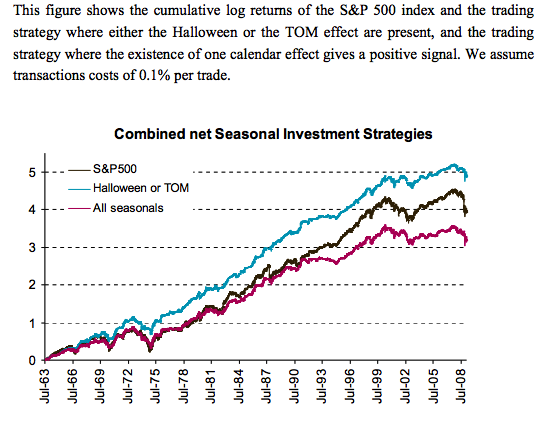
An excellent paper entitled An Anatomy of Calendar Effects in the Journal of Asset Management (13(4), 2012, pp. 271-286) by Laurens Swinkels of Erasmus University Rotterdam and Pim van Vliet of Robeco Asset Management gives a very good account of the various phenomena and their relative importance.  Using daily returns data on the US value-weighted equity market over the period from July 1963 to December 2008, the researchers find that Halloween and turn-of-the-month (TOM) are the strongest effects, fully diminishing the other three effects to zero. The equity premium over the sample 1963-2008 is 7.2% if there is a Halloween or TOM effect, and -2.8% in all other cases. These findings are robust with respect to transactions costs, across different samples, market segments, and international stock markets. Their empirical research narrows down the number of calendar effects from five to two, leading to a more powerful and puzzling summary of seasonal effects.

SSALGOTRADING AD

The two principal effects are illustrated here with reference to daily returns in the S&P 500 Index, using data from 1980-2016.
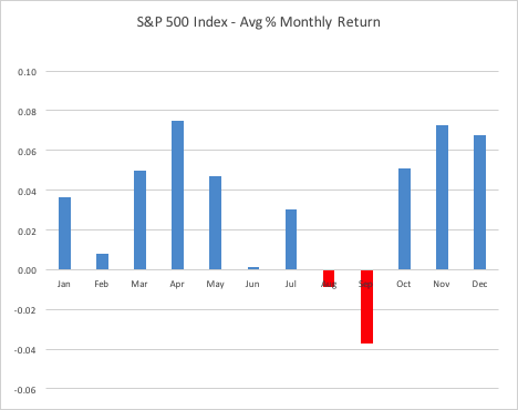
Halloween Effect

The Halloween effect refers to the tendency of markets to perform better in the six month period from November to April, compared to the half year from May to October.  In fact, for the S&P 500 index itself, performance during the months of May and October has historically been above the monthly average, as you can see in the chart below.  According to this analysis, the period to avoid spans the four months from June to September, with September being the “cruelest month”, by far.  Note that, between them, the months of November, December and April account for over 50% of the average annual return in the index since 1980.

Halloween Effect S&P500 Index


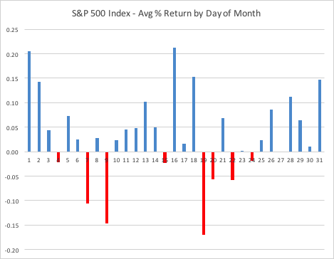
Turn-of-the-Month Effect

The TOM effect refers to the finding that above average returns tend to occur on the last trading day of the month and (up to) the first four trading days of the new calendar month. For the S&P 500 index the TOM effect spans a shorter period comprising the last trading day of the month and the first two trading days of the new month.  It is worth noting also the anomalous positive returns arising on 16th – 18th of the month and negative returns around the 19th and 20th of the month.    My speculative guess is that these mid-month effects arise from futures/option expiration.

TOM Effect S&P500 Index

Seasonal Tactical  Allocation

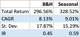
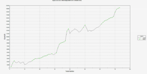
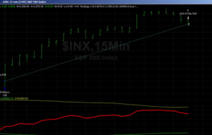
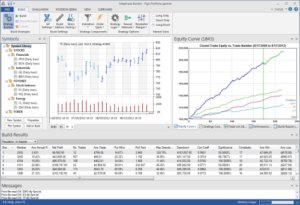
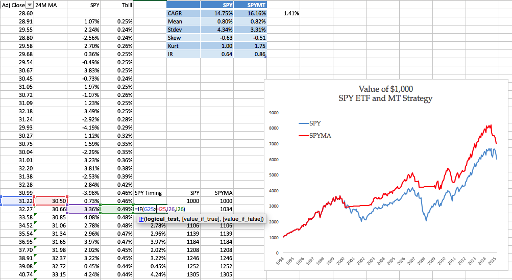
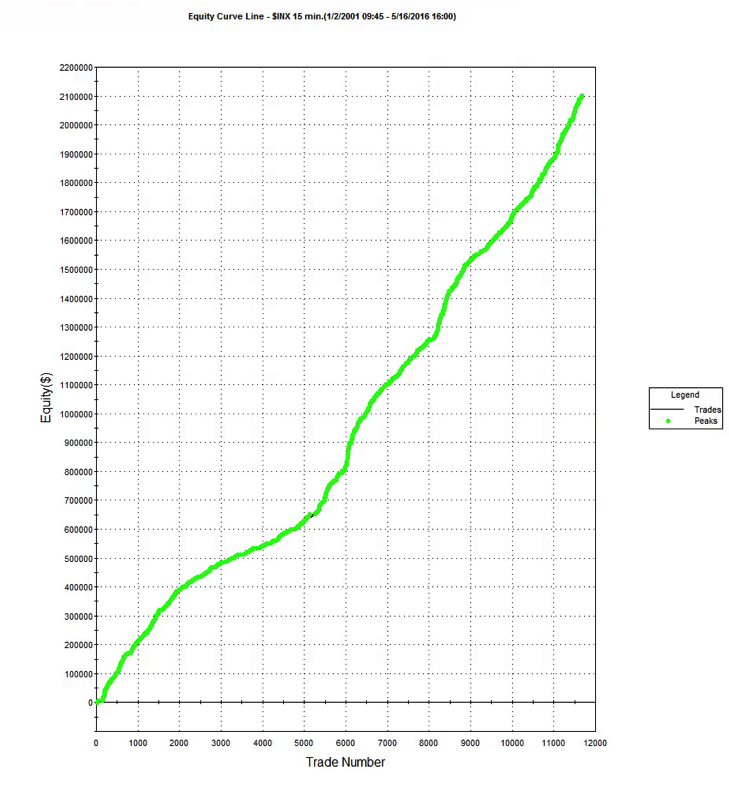
Let’s assume we allocate to equities (in the form of the S&P 500 Index) only during the period from October to May, or on the last or first two trading days of each month. How do the returns from that seasonal portfolio compare to the benchmark buy and hold portfolio?  If we ignore transaction costs (and income from riskless Treasury investments when we are out of the market), the seasonal portfolio outperforms the buy and hold benchmark over the 36 year period since 1980 by around 88bp per annum (continuously compounded), and with an annual volatility that is 258bp lower.  The outperformance of the seasonal portfolio becomes particularly noticeable after the 2000/2001 crash.


perfSeasonal


Seasonal vsB&H


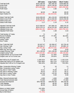
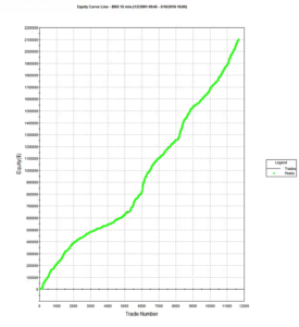
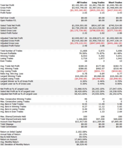
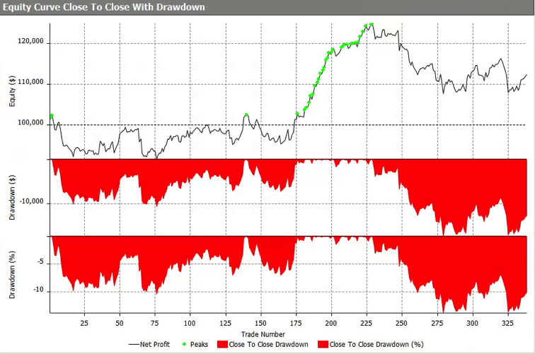
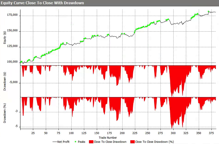
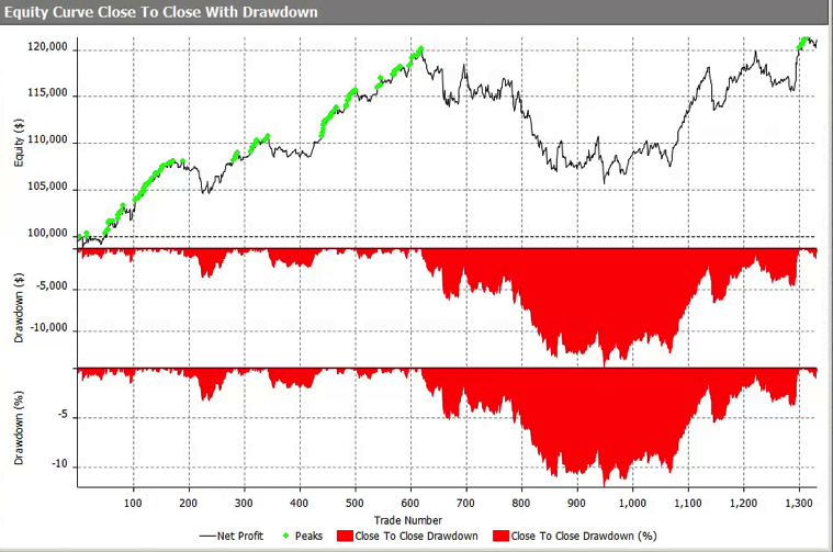
A much more rigorous analysis of the performance characteristics of the seasonal portfolio is given in the research paper, taking account of transaction costs, with summary results as follows:
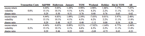
 

table 5


fig3

Conclusion

There is a sizable body of credible academic research demonstrating the importance of calendar effects and this paper suggests that investors’ focus should be on the Halloween and TOM effects in particular.  A tactical allocation program that increases the allocation to equities towards the end of the month and first few trading days of the new month, and during the November to April calendar months is likely to significantly outperform a buy-and-hold portfolio, according to these findings.

There remain unaccounted-for seasonal effects in the mid-section of the month that may arise from the expiration of futures and option contracts. These are worthy of further investigation.

Trading With Indices

In this post I want to discuss ways to make use of signals from relevant market indices in your trading.  These signals can add value regardless of whether you trade algorithmically or manually.  The techniques described here are one of the most widely applicable in the quantitative analyst’s arsenal.

Let’s motivate the discussion by looking an example of a simple trading system trading the VIX on weekly bars.  Performance results for the system are summarized in the chart and table below.  The system outperforms the buy and hold return by a substantial margin, with a profit factor of over 3 and a win rate exceeding 82%.  What’s not to like?

VIX EC

VIX Performance

Well, for one thing, this isn’t really a trading system – because the VIX Index itself isn’t tradable. So the performance results are purely notional (and, if you didn’t already notice, no slippage or commission is included).

It is very easy to build high-performing trading system in indices – because they are not traded products,  index prices are often stale and tend to “follow” the price action in the equivalent traded market.

This particular system for the VIX Index took me less than ten minutes to develop and comprises only a few lines of code.  The system makes use of a simple RSI indicator to decide when to buy or sell the index.  I optimized the indicator parameters (separately for long and short) over the period to 2012, and tested it out-of-sample on the data from 2013-2016.

inputs:
Price( Close ) ,
Length( 14 ) ,
OverSold( 30 ) ;

variables:
RSIValue( 0 );

RSIValue = RSI( Price, Length );
if CurrentBar > 1 and RSIValue crosses over OverSold then
Buy ( !( “RsiLE” ) ) next bar at market;

.

The daily system I built for the S&P 500 Index is a little more sophisticated than the VIX model, and produces the following results.

SP500 EC

SP500 Perf


Using Index Trading Systems

We have seen that its trivially easy to build profitable trading systems for index products.  But since they can’t be traded, what’s the point?

The analyst might be tempted by the idea of using the signals generated by an index trading system to trade a corresponding market, such as VIX or eMini futures.  However, this approach is certain to fail.  Index prices lag the prices of equivalent futures products, where traders first monetize their view on the market.  So using an index strategy directly to trade a cash or futures market would be like trying to trade using prices delayed by a few seconds, or minutes – a recipe for losing money.

SSALGOTRADING AD

Nor is it likely that a trading system developed for an index product will generalize to a traded market.  What I mean by this is that if you were to take an index strategy, such as the VIX RSI strategy, transfer it to VIX futures and tweak the parameters in the hope of producing a profitable system, you are likely to be disappointed. As I have shown, you can produce a profitable index trading system using the simplest and most antiquated trading concepts (such as the RSI index) that long ago ceased to offer any predictive value in actual traded markets.  Index markets are actually inefficient – the prices of index products often fail to fully reflect all relevant, available information in a timely way. Such simple inefficiencies are easily revealed by indicators such as moving averages.  Traded markets, by contrast, are highly efficient and, with the exception of HFT, it is going to take a great deal more than a simple moving average to provide insight into the few inefficiencies that do arise.

bullbear

Strategies in index products are best thought of, not as trading strategies, but rather as a means of providing broad guidance as to the general condition of the market and its likely direction over the longer term.  To take the VIX index strategy as an example, you can see that each “trade” spans several weeks.  So one might regard a “buy” signal from the VIX index system as an indication that volatility is expected to rise over the next month or two.  A trader might use that information to lean on the side of being long volatility, perhaps even avoiding any short volatility positions altogether for the next several weeks.  Following the model’s guidance in that way would would certainly have helped many equity and volatility traders during the market sell off during August 2015, for example:


Vix Example

The S&P 500 Index model is one I use to provide guidance as to market conditions for the current trading day.  It is a useful input to my thinking as to how aggressive I want my trading models to be during the upcoming session. If the index model suggests a positive tone to the market, with muted volatility, I might be inclined to take a more aggressive stance.  If the model starts trading to the short side, however, I am likely to want to be much more cautious.    Yesterday (May 16, 2016), for example, the index model took an early long trade, providing confirmation of the positive tenor to the market and encouraging me to trade volatility to the short side more aggressively.


SP500 Example


In general, I would tend to classify index trading systems as “decision support” tools that provide a means of shading opinion on the market, or perhaps providing a means of calibrating trading models to the anticipated market conditions. However, they can be used in a more direct way, short of actual trading.  For example, one of our volatility trading systems uses the trading signals from a trading system designed for the VVIX volatility-of-volatility index.  Another approach is to use the signals from an index trading system as an indicator of the market regime in a regime switching model.

Designing Index Trading Models

Whereas it is profitability that is typically the primary design criterion for an actual trading system, given the purpose of an index trading system there are other criteria that are at least as important.

It should be obvious from these few illustrations that you want to design your index model to trade less frequently than the system you are intending to trade live: if you are swing-trading the eminis on daily bars, it doesn’t help to see 50 trades a day from your index system.  What you want is an indication as to whether the market action over the next several days is likely to be positive or negative.  This means that, typically, you will design your index system using bar frequencies at least as long as for your live system.

Another way to slow down the signals coming from your index trading system is to design it for very high accuracy – a win rate of  70%, or higher.  It is actually quite easy to do this:  I have systems that trade the eminis on daily bars that have win rates of over 90%.  The trick is simply that you have to be prepared to wait a long time for the trade to come good.  For a live system that can often be a problem – no-one like to nurse an underwater position for days or weeks on end.  But for an index trading system it matters far less and, in fact, it helps:  because you want trading signals over longer horizons than the time intervals you are using in your live trading system.

Since the index system doesn’t have to trade live, it means of course that the usual trading costs and frictions do not apply.  The advantage here is that you can come up with concepts for trading systems that would be uneconomic in the real world, but which work perfectly well in the frictionless world of index trading.  The downside, however, is that this might lead you to develop index systems that trade far too frequently.  So, even though they should not apply, you might seek to introduce trading costs in order to penalize higher frequency trading systems and benefit systems that trade less frequently.

Designing index trading systems in an area in which genetic programming algorithms excel.  There are two main reasons for this.  Firstly, as I have previously discussed, simple technical indicators of the kind employed by GP modeling systems work well in index markets.  Secondly, and more importantly, you can use the GP system to tailor an index trading system to meet the precise criteria you have in mind, such as the % win rate, trading frequency, etc.

An outstanding product that I can highly recommend in this context is Mike Bryant’s Adaptrade Builder.  Builder is a superb piece of software whose power and ease of use reflects Mike’s engineering background and systems development expertise.


Adaptrade


Some Further Notes on Market Timing

Almost at the very moment I published a post featuring some interesting research by Glabadanidis (“Market Timing With Moving Averages”  (2015), International Review of Finance, Volume 15, Number 13, Pages 387-425 – see Yes, You Can Time the Market. How it Works, And Why), several readers wrote to point out a recently published paper by Valeriy Zakamulin, (dubbed the “Moving Average Research King” by Alpha Architect, the source for our fetching cover shot) debunking Glabadanidis’s findings in no uncertain terms:

We demonstrate that “too good to be true” reported performance of the moving average strategy is due to simulating the trading with look-ahead bias. We perform the simulations without look-ahead bias and report the true performance of the moving average strategy. We find that at best the performance of the moving average strategy is only marginally better than that of the corresponding buy-and-hold strategy.

So far, no response from Glabadanidis – from which one is tempted to conclude that Zakamulin is correct.

I can’t recall the last time a paper published in a leading academic journal turned out to be so fundamentally flawed.  That’s why papers are supposed to be peer reviewed.   But, I guess, it can happen. Still, it’s rather alarming to think that a respected journal could accept a piece of research as shoddy as Zakamulin claims it to be.

What Glabadanidis had done, according to Zakamulin, was to use the current month closing price to compute the moving average that was used to decide whether to exit the market (or remain invested) at the start of the same month.  An elementary error that introduces look-ahead bias that profoundly impacts the results.

Following this revelation I hastily checked my calculations for the SPY marketing timing  strategy illustrated in my blog post and, to my relief, confirmed that I had avoided the look-ahead trap that Glabadanidis has fallen into.  As the reader can see from the following extract from the Excel spreadsheet I used for the calculations, the decision to assume the returns for the SPY ETF or T-Bills for the current month rests on the value of the 24 month MA computed using prices up to the end of the prior month.  In other words, my own findings are sound, even if Glabadanidis’s are not, as the reader can easily check for himself.


Excel Workbook


Nonetheless, despite my relief at having avoided Glabadanidis’s  blunder, the apparent refutation of his findings comes as a disappointment.  And my own research on the SPY market timing strategy, while sound as far as it goes, cannot by itself rehabilitate the concept of market timing using moving averages.  The reason is given in the earlier post.  There is a hidden penalty involved in using the market timing strategy to synthetically replicate an Asian put option, namely the costs incurred in exiting and rebuilding the portfolio as the market declines below the moving average, or later overtakes it.  In a single instance, such as the case of SPY, it might easily transpire simply by random chance that the cost of replication are far lower than the fair value of the put.  But the whole point of Glabadanidis’s research was that the same was true, not only for a single ETF or stock, but for many thousands of them.  Absent that critical finding, the SPY case is no more than an interesting anomaly.

Finally, one reader pointed out that the effect of combining a put option with a stock (or ETF) long position was to create synthetically a call option in the stock (ETF).  He is quite correct.  The key point, however, is that when the stock trades down below its moving average, the value of the long synthetic call position and the market timing portfolio are equivalent.


The Information Content of the Pre- and Post-Market Trading Sessions

I apologize in advance for this rather “wonkish” post, which is aimed chiefly at the high frequency fraternity, or those at least who trade intra-day, in the equity markets.  Such minutiae are the lot of those engaged in high frequency trading.  I promise that my next post will be of more general interest.

Pre- and Post Market Sessions

The pre-market session in US equities runs from 8:00 AM ET, while the post-market session runs until 8:00 PM ET.  The question arises whether these sessions are worth trading, or at the very least, offer a source of data (quotes, trades) that might be relevant to trading the regular session, which of course runs from 9:30 AM to 4:00 PM ET.  Even if liquidity is thin and trades infrequent, and opportunities in the pre- and post-market very limited, it might be that we can improve our trading models by taking into account such information as these sessions do provide, even if we only ever plan to trade during regular trading hours.

It is somewhat challenging to discuss this in great detail, because HFT equity trading is very much in the core competencies of my firm, Systematic Strategies.  However, I hope to offer some ideas, at least, that some readers may find useful.

SSALGOTRADING AD


A Tale of Two Pharmaceutical Stocks

In what follows I am going to make use of two examples from the pharmaceutical industry: Alexion Pharmaceuticals, Inc. (ALXN), which has a market cap of $35Bn and trades around 800,000 shares daily, and Pfizer Inc. (PFE), which has a market cap of over $200Bn and trades close to 50M shares a day.

Let’s start by looking at a system trading ALXN during regular market hours.  The system isn’t high frequency, but trades around 1-2 times a day, on average.  The strategy equity curve from 2015 to April 2016 is not at all impressive.


ALXN Regular

ALXN – Regular Session Only


But look at the equity curve for the same strategy when we allow it to run on the pre- and post-market sessions, in addition to regular trading hours.  Clearly the change in the trading hours utilized by the strategy has made a huge improvement in the total gain and risk-adjusted returns.


ALEXN with pre-market

ALXN – with Pre- and Post-Market Sessions


The PFE system trades much more frequently, around 4 times a day, but the story is somewhat similar in terms of how including the pre- and post-market sessions appears to improve its performance.

PFE Regular

PFE – Regular Session Only

PFE with premarket

PFE – with Pre- and Post-Market Sessions


Improving Trading Performance

In both cases, clearly, the trading performance of the strategies has improved significantly with the inclusion of the out-of-hours sessions.  In the case of ALXN, we see a modest increase of around 10% in the total number of trades, but in the case of PFE the increase in trading activity is much more marked – around 30%, or more.

The first important question to ask is when these additional trades are occurring.  Assuming that most of them take place during the pre- or post-market, our concern might be whether there is likely to be sufficient liquidity to facilitate trades of the frequency and size we wish to execute.  Of various possible hypotheses, some negative, other positive, we might consider the following:

(a) Bad ticks in the market data feed during out-of-hours sessions give rise to apparently highly profitable “phantom” trades

(b) The market data is valid, but the trades are done in such low volume as to be insignificant for practical purposes (i.e. trades were done for a few hundred lots and additional liquidity is unlikely to be available)

(c) Out-of-hours sessions enable the system to improve profitability by entering or exiting positions in a more timely manner than by trading the regular session alone

(d) Out-of-hours market data improves the accuracy of model forecasts, facilitating a larger number of trades, and/or more profitable trades, during regular market hours

An analysis of the trading activity for the two systems provides important insight as to which of the possible explanations might be correct.


ALXN Analysis

(click to enlarge)

Dealing first with ALXN, we that, indeed, an additional 11% of trades are entered or exited out-of-hours.  However, these additional trades account for somewhere between 17% (on exit) and 20% (on entry) of the total profits.  Furthermore, the size of the average entry trade during the post-market session and of the average exit trade in the pre-market session is more than double that of the average trade entered or exited during regular market hours. That gives concerns that some of the apparent increase in profits may be due to bad ticks at prices away from the market, allowing the system enter or exit trades at unrealistically low or high prices.  Even if many of the trades are good, we will have concerns about the scalability of the strategy in out-of-hours trading, given the relatively poor liquidity in the stock. On the other hand, at least some of the uplift in profits arises from new trades occurring during the regular session. This suggests that, even if we are unable to execute many of the trading opportunities seen during pre- or post-market, the trades from those sessions provides useful additional data points for our model, enabling it to increase the number and/or profitability of trades in the regular session.

Next we turn to PFE.  We can see straight away that, while the proportion of trades occurring during out-of-hours sessions is around 23%, those trades now account for over 50% of the total profits.  Furthermore, the average PL for trades executed on entry post-market, and on exit pre-market, is more than 4x the average for trades entered or exited during normal market hours.  Despite the much better liquidity in PFE compared to ALXN, this is a huge concern – we might expect to see significant discrepancies occurring between theoretical and actual performance of the strategy, due to the very high dependency on out-of-hours trading.

PFE Analysis

(click to enlarge)

As we dig further into the analysis, we do indeed find evidence that bad data ticks play a disproportionate role.  For example, this trade in PFE which apparently occurred at around 16:10 on 4/6 was almost certainly a phantom trade resulting from a bad data point. It turns out that, for whatever reason, such bad ticks are a common occurrence in the stock and account for a large proportion of the apparent profitability of out-of-hours trading in PFE.


PFE trade


CONCLUSION

We are, of course, only skimming the surface of the analysis that is typically carried out.  One would want to dig more deeply into ways in which the market data feed could be cleaned up and bad data ticks filtered out so as to generate fewer phantom trades.  One would also want to look at liquidity across the various venues where the stocks trade, including dark pools, in order to appraise the scalability of the strategies.

For now, the main message that I am seeking to communicate is that it is often well worthwhile considering trading in the pre- and post-market sessions, not only with a view to generating additional, profitable trading opportunities, but also to gather additional data points that can enhance trading profitability during regular market hours.