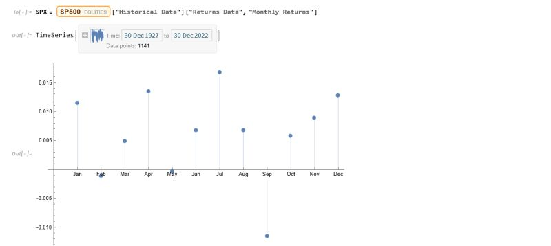
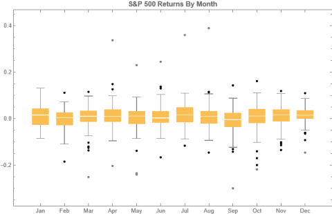
To amplify Valérie Noël‘s post a little, we can use the Equities Entity Store (https://lnkd.in/epg-5wwM) to extract returns for the S&P500 index for (almost) the last century and compute the average return by month, as follows.
July is shown to be (by far) the most positive month for the index, with an average return of +1.67%, in stark contrast to the month of Sept. in which the index has experienced an average negative return of -1.15%.
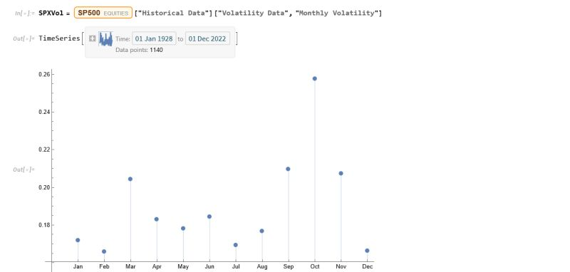
Continuing the analysis a little further, we can again use the the Equities Entity Store (https://lnkd.in/epg-5wwM) to extract estimated average volatility for the S&P500 by calendar month since 1927:
As you can see, July is not only the month with highest average monthly return, but also has amongst the lowest levels of volatility, on average.
Consequently, risk-adjusted average rates of return in July far exceed other months of the year.
Conclusion: bears certainly have a case that the market is over-stretched here, but I would urge caution: hold off until end Q3 before shorting this market in significant size.
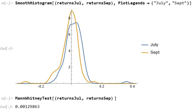
For those market analysts who prefer a little more analytical meat, we can compare the median returns for the #S&P500 Index for the months of July and September using the nonparametric MannWhitney test.
This indicates that there is only a 0.13% probability that the series of returns for the two months are generated from distributions with the same median.
Conclusion: Index performance in July really is much better than in September.
For more analysis along these lines, see my recent book, Equity Analytics:
One of the main criticisms levelled at systematic trading over the last few years is that the over-use of historical market data has tended to produce curve-fitted strategies that perform poorly out of sample in a live trading environment. This is indeed a valid criticism – given enough attempts one is bound to arrive eventually at a strategy that performs well in backtest, even on a holdout data sample. But that by no means guarantees that the strategy will continue to perform well going forward.
The solution to the problem has been clear for some time: what is required is a method of producing synthetic market data that can be used to build a strategy and test it under a wide variety of simulated market conditions. A strategy built in this way is more likely to survive the challenge of live trading than one that has been developed using only a single historical data path.
The problem, however, has been in implementation. Up until now all the attempts to produce credible synthetic price data have failed, for one reason or another, as I described in an earlier post:
I have been able to devise a completely new algorithm for generating artificial price series that meet all of the key requirements, as follows:
Computational simplicity & efficiency. Important if we are looking to mass-produce synthetic series for a large number of assets, for a variety of different applications. Some deep learning methods would struggle to meet this requirement, even supposing that transfer learning is possible.
The ability to produce price series that are internally consistent (i.e High > Low, etc) in every case .
Should be able to produce a range of synthetic series that vary widely in their correspondence to the original price series. In some case we want synthetic price series that are highly correlated to the original; in other cases we might want to test our investment portfolio or risk control systems under extreme conditions never before seen in the market.
The distribution of returns in the synthetic series should closely match the historical series, being non-Gaussian and with “fat-tails”.
The ability to incorporate long memory effects in the sequence of returns.
The ability to model GARCH effects in the returns process.
This means that we are now in a position to develop trading strategies without any direct reference to the underlying market data. Consequently we can then use all of the real market data for out-of-sample back-testing.
Developing a Trading Strategy for the S&P 500 Index Using Synthetic Market Data
To illustrate the procedure I am going to use daily synthetic price data for the S&P 500 Index over the period from Jan 1999 to July 2022. Details of the the characteristics of the synthetic series are given in the post referred to above.
Because we want to create a trading strategy that will perform under market conditions close to those currently prevailing, I will downsample the synthetic series to include only those that correlate quite closely, i.e. with a minimum correlation of 0.75, with the real price data.
Why do this? Surely if we want to make a strategy as robust as possible we should use all of the synthetic data series for model development?
The reason is that I believe that some of the more extreme adverse scenarios generated by the algorithm may occur quite rarely, perhaps once in every few decades. However, I am principally interested in a strategy that I can apply under current market conditions and I am prepared to take my chances that the worst-case scenarios are unlikely to come about any time soon. This is a major design decision, one that you may disagree with. Of course, one could make use of every available synthetic data series in the development of the trading model and by doing so it is likely that you would produce a model that is more robust. But the training could take longer and the performance during normal market conditions may not be as good.
Having generated the price series, the process I am going to follow is to use genetic programming to develop trading strategies that will be evaluated on all of the synthetic data series simultaneously. I will then use the performance of the aggregate portfolio, i.e. the outcome of all of the trades generated by the strategy when applied to all of the synthetic series, to assess the overall performance. In order to be considered, candidate strategies have to perform well under all of the different market scenarios, or at least the great majority of them. This ensures that the strategy is likely to prove more robust across different types of market conditions, rather than on just the single type of market scenario observed in the real historical series.
As usual in these cases I will reserve a portion (10%) of each data series for testing each strategy, and a further 10% sample for out-of-sample validation. This isn’t strictly necessary: since the real data series has not be used directly in the development of the trading system, we can later test the strategy on all of the historical data and regard this as an out-of-sample backtest.
To implement the procedure I am going to use Mike Bryant’s excellent Adaptrade Builder software.
This is an exemplar of outstanding software engineering and provides a broad range of features for generating trading strategies of every kind. One feature of Builder that is particularly useful in this context is its ability to construct strategies and test them on up to 20 data series concurrently. This enables us to develop a strategy using all of the synthetic data series simultaneously, showing the performance of each individual strategy as well for as the aggregate portfolio.
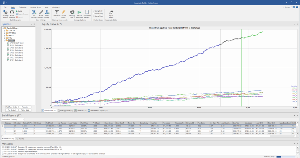
After evolving strategies for 50 generations we arrive at the following outcome:
The equity curve for the aggregate portfolio is shown in blue, while the equity curves for the strategy applied to individual synthetic data series are shown towards the bottom of the chart. Of course, the performance of the aggregate portfolio appears much superior to any of the individual strategies, because it is effectively the arithmetic sum of the individual equity curves. And just because the aggregate portfolio appears to perform well both in-sample and out-of-sample, that doesn’t imply that the strategy works equally well for every individual market scenario. In some scenarios it performs better than in others, as can be observed from the individual equity curves.
But, in any case, our objective here is not to create a stock portfolio strategy, but rather to trade a single asset – the S&P 500 Index. The role of the aggregate portfolio is simply to suggest that we may have found a strategy that is sufficiently robust to work well across a variety of market conditions, as represented by the various synthetic price series.
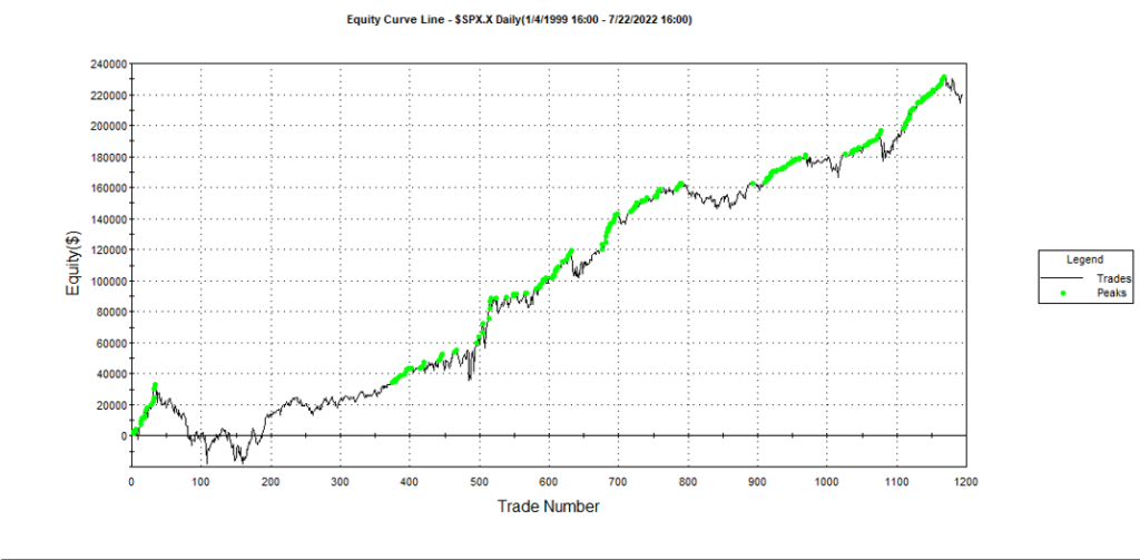
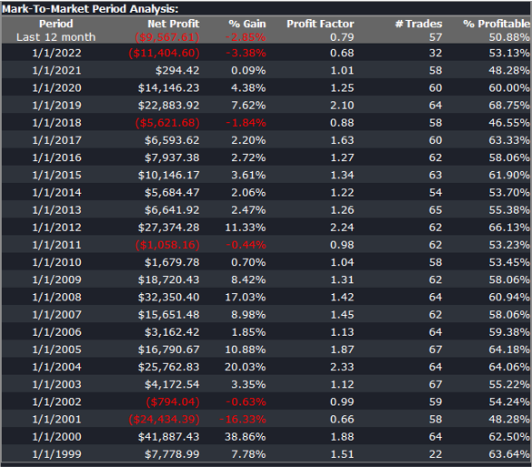
Builder generates code for the strategies it evolves in a number of different languages and in this case we take the EasyLanguage code for the fittest strategy #77 and apply it to a daily chart for the S&P 500 Index – i.e. the real data series – in Tradestation, with the following results:
The strategy appears to work well “out-of-the-box”, i,e, without any further refinement. So our quest for a robust strategy appears to have been quite successful, given that none of the 23-year span of real market data on which the strategy was tested was used in the development process.
We can take the process a little further, however, by “optimizing” the strategy. Traditionally this would mean finding the optimal set of parameters that produces the highest net profit on the test data. But this would be curve fitting in the worst possible sense, and is not at all what I am suggesting.
Instead we use a procedure known as Walk Forward Optimization (WFO), as described in this post:
The goal of WFO is not to curve-fit the best parameters, which would entirely defeat the object of using synthetic data. Instead, its purpose is to test the robustness of the strategy. We accomplish this by using a sequence of overlapping in-sample and out-of-sample periods to evaluate how well the strategy stands up, assuming the parameters are optimized on in-sample periods of varying size and start date and tested of similarly varying out-of-sample periods. A strategy that fails a cluster of such tests is unlikely to prove robust in live trading. A strategy that passes a test cluster at least demonstrates some capability to perform well in different market regimes.
To some extent we might regard such a test as unnecessary, given that the strategy has already been observed to perform well under several different market conditions, encapsulated in the different synthetic price series, in addition to the real historical price series. Nonetheless, we conduct a WFO cluster test to further evaluate the robustness of the strategy.
As the goal of the procedure is not to maximize the theoretical profitability of the strategy, but rather to evaluate its robustness, we select a criterion other than net profit as the factor to optimize. Specifically, we select the sum of the areas of the strategy drawdowns as the quantity to minimize (by maximizing the inverse of the sum of drawdown areas, which amounts to the same thing). This requires a little explanation.
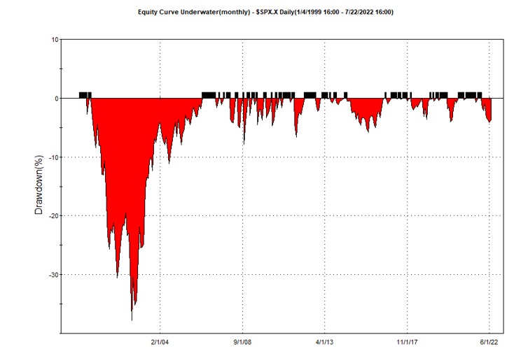
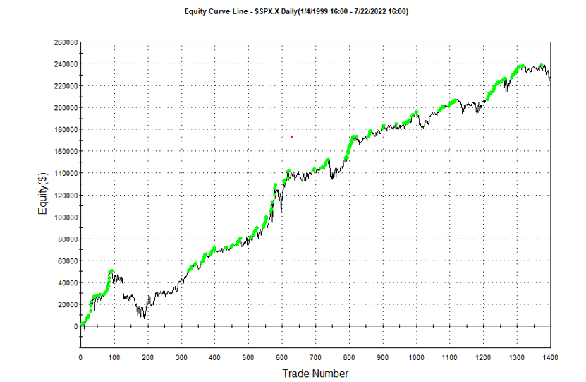
If we look at the strategy drawdown periods of the equity curve, we observe several periods (highlighted in red) in which the strategy was underwater:
The area of each drawdown represents the length and magnitude of the drawdown and our goal here is to minimize the sum of these areas, so that we reduce both the total duration and severity of strategy drawdowns.
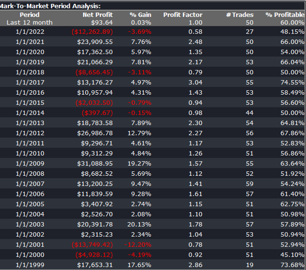
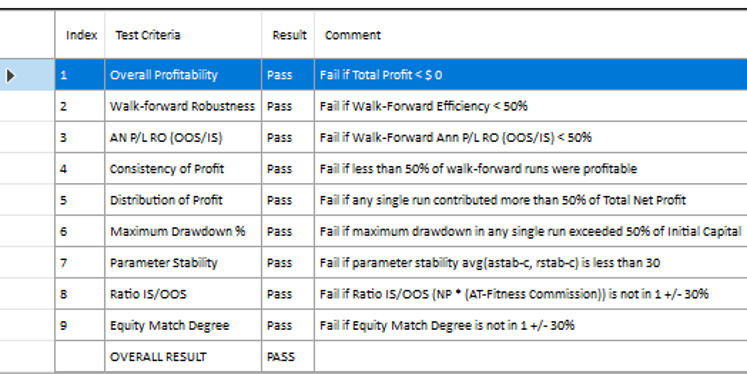
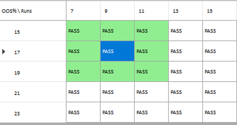
In each WFO test we use different % of OOS data and a different number of runs, assessing the performance of the strategy on a battery of different criteria:
x
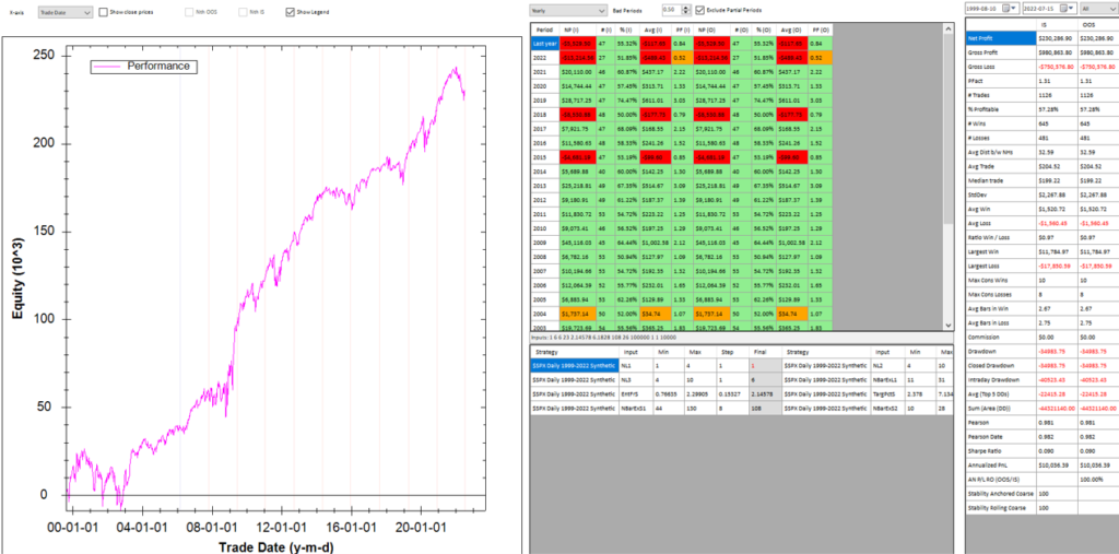
These criteria not only include overall profitability, but also factors such as parameter stability, profit consistency in each test, the ratio of in-sample to out-of-sample profits, etc. In other words, this WFO cluster analysis is not about profit maximization, but robustness evaluation, as assessed by these several different metrics. And in this case the strategy passes every test with flying colors:
Other than validating the robustness of the strategy’s performance, the overall effect of the procedure is to slightly improve the equity curve by diminishing the magnitude and duration of the drawdown periods:
Conclusion
We have shown how, by using synthetic price series, we can build a robust trading strategy that performs well under a variety of different market conditions, including on previously “unseen” historical market data. Further analysis using cluster WFO tests strengthens the assessment of the strategy’s robustness.
The principal argument in favor of using synthetic data is that it addresses one of the major concerns about using real data series for modelling purposes: i.e. that models designed to fit the historical data produce test results that are unlikely to be replicated, going forward. Such models are not robust to changes that are likely to occur in any dynamical statistical process and will consequently perform poorly out of sample.
By using multiple synthetic data series following a wide range of different price paths, one can hope to build models – both for risk management and investment purposes – that can accommodate a variety of different market scenarios, making them more likely to perform robustly in a live market context.
Producing authentic synthetic data is a significant challenge, one that has eluded researchers for many years. Generating artificial returns series is a considerably simpler task, but even here there are difficulties. For many applications it is simply not sufficient to sample from the empirical distribution, because we want to produce a sequence of returns that closely mirrors the pattern of real returns sequences. In particular, there may be long memory effects (non-zero autocorrelations at long lags) or GARCH effects, in which dependency is introduced into the returns process via the square (or absolute value) of returns. These have the effect of inducing “shocks” to the returns process that persist for some time, causing autocorrelation in the associated volatility process in the process.
But producing a set of synthetic stock price data is even more of a challenge because not only do the above do the above requirements apply, but we also need to ensure that the open, high, low and closing prices are internally consistent, i.e. that on any given bar the High >= {Open, Low and Close) and that the Low <= {Open, Close}. These basic consistency checks have been overlooked in the research thus far.
Econometric Methods
One classical approach to the problem would be to create a Vector Autoregression Model, in which lagged values of the Open, High, Low and Close prices are used to predict the current values (see here for a detailed exposition of the VAR approach). A compelling argument in favor of such models is that, almost by definition, O/H/L/C prices are necessarily cointegrated.
While a VAR model potentially has the ability to model long memory and even GARCH effects, it is unable to produce stock prices that are guaranteed to be consistent, in the sense defined above. Indeed, a failure rate of 35% or higher for basic consistency checks is typical for such a model, making the usefulness of the synthetic prices series highly questionable.
Another approach favored by some researchers is to stitch together sub-samples of the real data series in a varying time-order. This is applicable only to return series and, in any case, can introduce spurious autocorrelations, or overlook important dependencies in the data series. Besides these defects, it is challenging to produce a synthetic series that looks substantially different from the original – both the real and synthetic series exhibit common peaks and troughs, even if they occur in different places in each series.
Deep Learning Generative Adversarial Networks
In a previous post I looked in some detail at TimeGAN, one of the more recent methods for producing synthetic data series introduced in a paper in 2019 by Yoon, et al (link here).
TimeGAN, which applies deep learning Generative Adversarial Networks to create synthetic data series, appears to work quite well for certain types of time series. But in my research I found it be inadequate for the purpose of producing synthetic stock data, for three reasons:
(i) The model produces synthetic data of fixed window lengths and stitching these together to form a single series can be problematic.
(ii) The prices fail a significant percentage of the basic consistency tests, regardless of the number of epochs used to train the model
(iii) The methodology introduces spurious correlations in the associated returns process that do not correspond to anything found in real stock return series and which get more pronounced as training continues.
Another GAN model, DoppleGANger, introduced by Lin, et. al. in 2020 (paper here) seeks to improve on TimeGAN and claims “up to 43% better fidelity than baseline models”, including TimeGAN. However, in my research I found that, while DoppleGANger trains much more quickly than TimeGAN, it produces a consistency test failure rate exceeding 30%, even after training for 500,000 epochs.
For both TimeGAN and DoppleGANger, the researchers have tended to benchmark performance using classical data science metrics such as TSNE plots rather than the more prosaic consistency checks that a market data specialist would be interested in, while the more advanced requirements such as long memory and GARCH effects are passed by without a mention.
The conclusion is that current methods fail to provide an adequate means of generating synthetic price series for financial assets that are consistent and sufficiently representative to be practically useful.
The Ideal Algorithm for Producing Synthetic Data Series
What are we looking for in the ideal algorithm for generating stock prices? The list would include:
(i) Computational simplicity & efficiency. Important if we are looking to mass-produce synthetic series for a large number of assets, for a variety of different applications. Some deep learning methods would struggle to meet this requirement, even supposing that transfer learning is possible.
(ii) The ability to produce price series that are internally consistent (i.e High > Low, etc) in every case .
(iii) Should be able to produce a range of synthetic series that vary widely in their correspondence to the original price series. In some case we want synthetic price series that are highly correlated to the original; in other cases we might want to test our investment portfolio or risk control systems under extreme conditions never before seen in the market.
(iv) The distribution of returns in the synthetic series should closely match the historical series, being non-Gaussian and with “fat-tails”.
(v) The ability to incorporate long memory effects in the sequence of returns.
(vi) The ability to model GARCH effects in the returns process.
After researching the problem over the course of many years, I have at last succeeded in developing an algorithm that meets these requirements. Before delving into the mechanics, let me begin by illustrating its application.
Application of the Ideal Algorithm
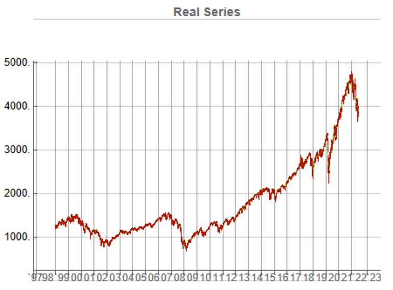
In this demonstration I am using daily O/H/L/C prices for the S&P 500 index for the period from Jan 1999 to July 2022, comprising four price series over 5,297 daily periods.
Synthetic Price Series
Generating ten synthetic series using the algorithm takes around 2 seconds with parallelization. I chose to generate series of the same length as the original, although I could just as easily have produced shorter, or longer sequences.
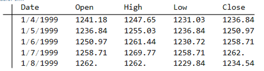
The first task is to confirm that the synthetic data are internally consistent, and indeed is guaranteed to be so because of the way the algorithm is designed. For example, here are the first few daily bars from the first synthetic series:
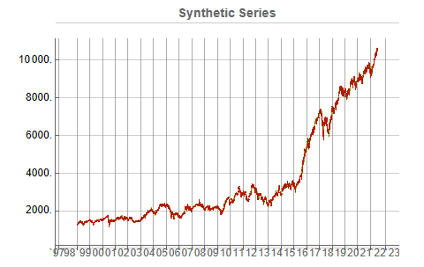
This means, of course, that we can immediately plot the synthetic series in a candlestick chart, just as we did with the real data series, above.
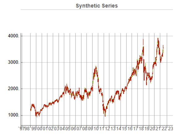
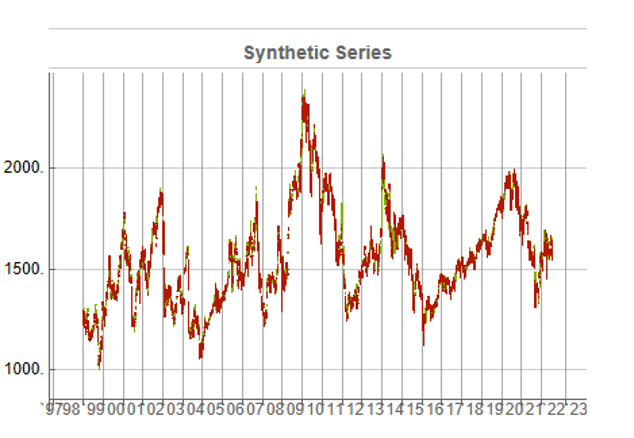
While the real and synthetic series are clearly different, the pattern of peaks and troughs somehow looks recognizably familiar. So, too, is the upward drift in the series, which is this case carries the synthetic S&P 500 Index to a high above 10,000 in 2022. Obviously this is a much more bullish scenario that we have seen in reality. But in fact this is just one example taken from the more “optimistic” end of the spectrum of possibilities. An illustration from the opposite end of the spectrum is shown in the chart below, in which the Index moves sideways over the entire 23 year span, with several very large drawdowns of -20% or more:
A more typical scenario might look something like our third chart, below. Here, too, we see several very large drawdowns, especially in the period from 2010-2011, but there is also a general upward drift in the process that enables the Index to reach levels comparable to those achieved by the real series:
Price Correlations
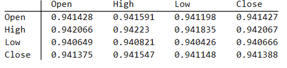
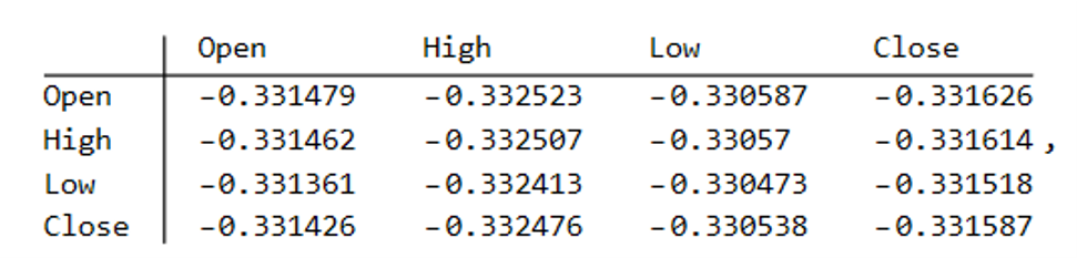
Reflecting these very different price path evolutions, we observe large variation in the correlations between the real and synthetic price series. For example:
As these tables indicate, the algorithm is capable of producing replica series that either mimic the original, real price series very closely, or which show completely different behavior, as in the second example.
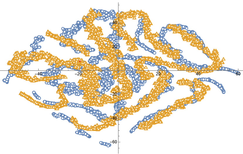
Dimensionality Reduction
For completeness, as have previous researchers, we apply t-SNE dimensionality reduction and plot the two-factor weightings for both real (yellow) and synthetic data (blue). We observe that while there is considerable overlap in reduced dimensional space, it is not as pronounced as for the synthetic data produced by TimeGAN, for instance. However, as previously explained, we are less concerned by this than we are about the tests previously described, which in our view provide a more appropriate analysis benchmark, so far as market data is concerned. Furthermore, for the reasons previously given, we want synthetic market data that in some cases tracks well beyond the range seen in historical price series.
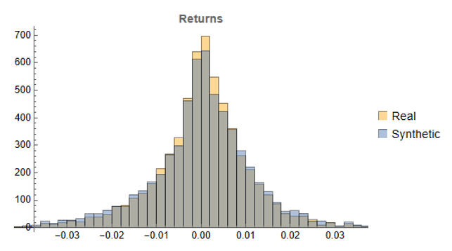
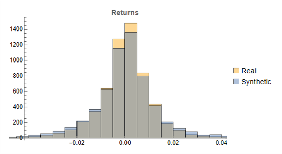
Returns Distributions
Moving on, we next consider the characteristics of the returns in the synthetic series in comparison to the real data series, where returns are measured as the differences in the Log-Close prices, in the usual way.
Histograms of the returns for the most “optimistic” and “pessimistic” scenarios charted previously are shown below:
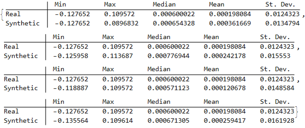
In both cases the distribution of returns in the synthetic series closely matches that of the real returns process and are clearly non-Gaussian, with an over-weighting in the distribution tails. A more detailed look at the distribution characteristics for the first four synthetic series indicates that there is a very good match to the real returns process in each case (the results for other series are very similar):
We observe that the minimum and maximum returns of the synthetic series sometimes exceed those of the real series, which can be a useful characteristic for risk management applications. The median and mean of the real and synthetic series are broadly similar, sometimes higher, in other cases lower. Only for the standard deviation of returns do we observe a systematic pattern, in which returns volatility in the synthetic series is consistently higher than in the real series.
This feature, I would argue, is both appropriate and useful. Standard deviations should generally be higher, because there is indeed greater uncertainty about the prices and returns in artificially generated synthetic data, compared to the real series. Moreover, this characteristic is useful, because it will impose a greater stress-test burden on risk management systems compared to simply drawing from the distribution of real returns using Monte Carlo simulation. Put simply, there will be a greater number of more extreme tail events in scenarios using synthetic data, and this will cause risk control parameters to be set more conservatively than they otherwise might. This same characteristic – the greater variation in prices and returns – will also pose a tougher challenge for AI systems that attempt to create trading strategies using genetic programming, meaning that any such strategies are more likely to perform robustly in a live trading environment. I will be returning to this issue in a follow-up post.
Returns Process Characteristics
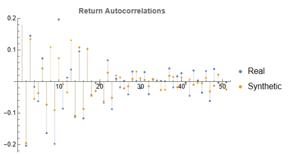
In the following plot we take a look at the autocorrelations in the returns process for a typical synthetic series. These compare closely with the autocorrelations in the real returns series up to 50 lags, which means that any long memory effects are likely to be conserved.
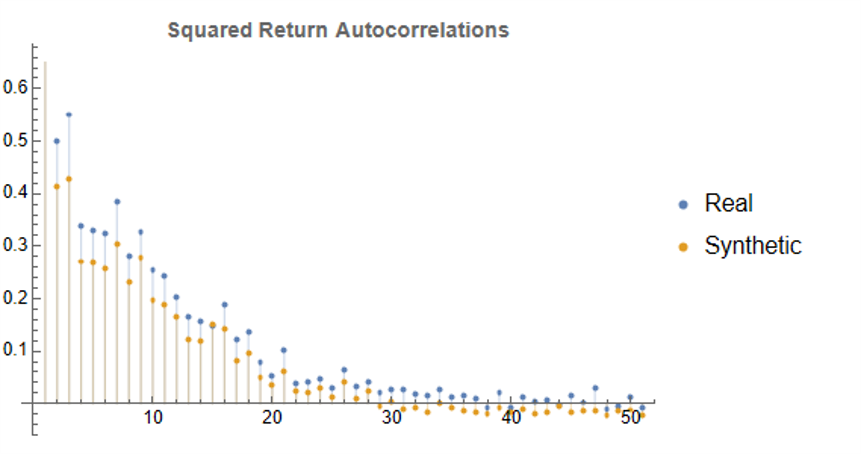
Finally, when we come to consider the autocorrelations in the square of the returns, we observe slowly decaying coefficients over long lags – evidence of so-called GARCH effects – for both real and synthetic series:
Summary
Overall, we observe that the algorithm is capable of generating consistent stock price series that correlate highly with the real price series. It is also capable of generating price series that have low, or even negative, correlation, a feature that may have important applications in the context of risk management. The distribution of returns in the synthetic series closely match those of the real returns process, and moreover retain important features such as long memory and GARCH effects.
Objections to the Use of Synthetic Data
Criticism of synthetic market data (including from myself) has hitherto focused on the inadequacy of such data in terms of representing important characteristics of real data series. Now that such technical issues have been addressed, I will try to anticipate some of the additional concerns that are likely to surface, going forward.
The Synthetic Data is “Unrealistic”
What is meant here is that there is no plausible set of real, economic factors that would be likely to combine in a way to produce the pattern of prices shown in some of the synthetic data series. The idea that, as observed in one of the artificial scenarios above, the Fed would stand idly by while the market plunged by 50% to 60%, seems highly implausible. Equally unlikely is a scenario in which the market moves sideways for an extended period of a decade, or longer.
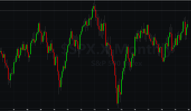
To a limited extent, I would agree with this. However, just because such scenarios are currently unlikely doesn’t mean they can never happen. For instance, take a look at the performance of the S&P 500 Index over the period from 1966 through 1979:
The market index barely made any progress throughout the entire 13-year period, which was characterized by a vicious bout of stagflation. Note, too, the precipitous drop in the index following the oil shock in 1973.
So to say that such scenarios – however implausible they may appear to be – can never happen is simply mistaken.
Finally, let’s not forget that, while the focus of this article is on the US market index, there are many economies, such as Mexico, Brazil or Argentina, for which such adverse developments are much more credible than they might currently be for the United States. We may wish to produce synthetic data for the markets in such economies for modelling purposes, in which case we will want to generate synthetic data capturing the full range of possible market outcomes, including some of the worst-case scenarios.
2. Extreme Scenarios Occur Too Frequently in Synthetic Data
Actually this is not the case – the generator tends to produce extreme scenarios with a frequency that is plausible, given the history and characteristics of the underlying, real price process. But there can be good reasons for wanting to control the frequency of such scenarios.
For instance, an investment manager may be looking to develop a “long-only” investment portfolio because, given his investment remit, that is the only type of investment strategy permitted. He would likely want to limit his focus to the more benign market outcomes for two reasons: (i) his investment thesis is that the market is likely to perform well, going forward (or else how does he pitch his strategy to investors?) and (ii) while he accepts that he may be wrong, it is not his job to hedge a possible market downturn – the responsibility for dealing with an adverse outcome falls to his risk manager, or to the investor.
Conversely, a risk manager is much more likely to be interested in adverse scenarios and, if anything, is likely to want to see such outcomes over-represented in a sample of synthetic data.
The point is, there is no “correct” answer: one has to decide which types of scenarios best suit the application one has in mind and sample the data accordingly. This can be done in a variety of ways such as setting a minimum required correlation between the synthetic and real price series, or designing a system of stratified sampling in which the desired outcomes are sampled according to a stipulated frequency distribution.
3. Synthetic Data Does Not Prevent Data Snooping and Curve Fitting
A critic might argue that, in fact, the real market data is “unseen” only in a theoretical sense, since its essential attributes have been baked into the synthetic series produced by the generator. This applies to an even greater extent if the synthetic series are sampled in some way, as described above.
I think this is a fair point. To take an extreme scenario, one could choose to select only synthetic series for which the correlation with the real data is 99.9%, or higher. Clearly this runs counter to the spirit of what one is trying to achieve with synthetic data and one might just as well use real data for modelling purposes. In practice, of course, even where a sampling methodology is applied, it is unlikely to be as crudely biased as in this example.
But, in any case, what is the alternative? The only option I can see is one in which a pure mathematical model is used to produce synthetic data, without any reference to the underlying real series. But, in that case, how would one assess the validity of the model assumptions, or how representative the synthetic series it produces might be?
There is no alternative but to have recourse to the real data at some point in the modelling process. In this procedure, however, the impact of snooping bias or curve fitting, even though it can never be totally extinguished, is very much diminished and it plays a less central role in model development.
Conclusion
It is now possible to produce synthetic data series that have all of the hallmark characteristics of real price data. This permits the analyst to investigate market models without direct recourse to the real price series, thereby minimizing data snooping and curve fitting bias. Models developed using synthetic data describing many different price path evolutions are more likely to prove robust across a wider range of plausible market scenarios in the real world.
In the next, follow-up post I will illustrate the application of synthetic data to the development of a robust investment strategy.
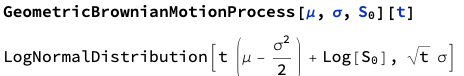
To recap briefly, we assume a process of the form:
Where S0 is the initial stock price at time t = 0.
The mean of such a process is:
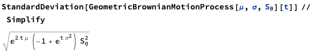
and standard deviation:
In the post I showed how to estimate such a process with daily stock prices, using these to provide a forecast range of prices over a one-month horizon. This is potentially useful, for example, in choosing which strikes to select in an option hedge.
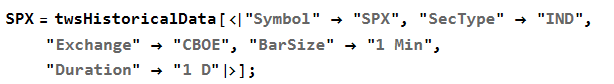
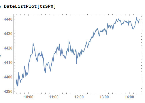
Of course, there is nothing to prevent you from using the same technique over different timescales. Here I use the MATH-TWS package to connect Mathematica to the IB TWS platform via the C++ api, to extract intraday prices for the S&P 500 Index at 1-minute intervals. These are used to estimate a short-term GBM process, which provides forecasts of the mean and variance of the index at the 4 PM close.
We capture the data using:
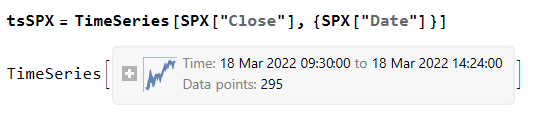
then create a time series of the intraday prices and plot them:
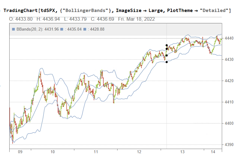
If we want something a little fancier we can create a trading chart, including technical indicators of our choice, for instance:
The charts can be updated in real time from IB, using MATHTWS.
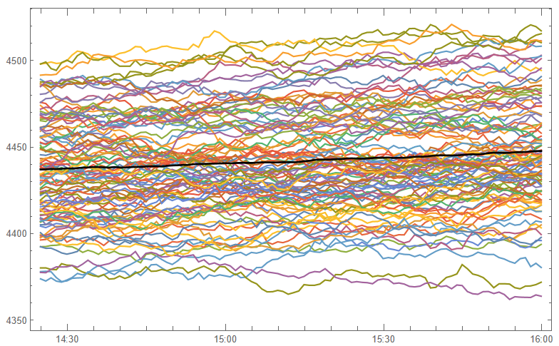
From there we estimate a GBM process using 1-minute close prices:
and then simulate a number of price paths towards the 4 PM close (the mean price path is shown in black):
This indicates that the expected value of the SPX index at the close will be around 4450, which we could estimate directly from:
Where u is the estimated drift of the GBM process.
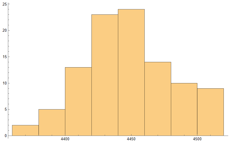
Similarly we can look at the projected terminal distribution of the index at 4pm to get a sense of the likely range of closing prices, which may assist a decision to open or close certain option (hedge) positions:
Of course, all this is predicated on the underlying process continuing on its current trajectory, with drift and standard deviation close to those seen in the process in the preceding time interval. But trends change, as do volatilities, which means that our forecasts may be inaccurate. Furthermore, the drift in asset processes tends to be dominated by volatility, especially at short time horizons.
So the best way to think of this is as a conditional expectation, i.e. “If the stock price continues on its current trajectory, then our expectation is that the closing price will be in the following range…”.
I have always been an advocate of incorporating index data into one’s trading strategies. Since they are not tradable, the “market” in index products if often highly inefficient and displays easily identifiable patterns that can be exploited by a trader, or a trading system. In fact, it is almost trivially easy to design “profitable” index trading systems and I gave a couple of examples in the post below, including a system producing stellar results in the S&P 500 Index.
Of course such systems are not directly useful. But traders often use signals from such a system as a filter for an actual trading system. So, for example, one might look for a correlated signal in the S&P 500 index as a means of filtering trades in the E-Mini futures market or theSPDR S&P 500 ETF (SPY).
Multi-Strategy Trading Systems
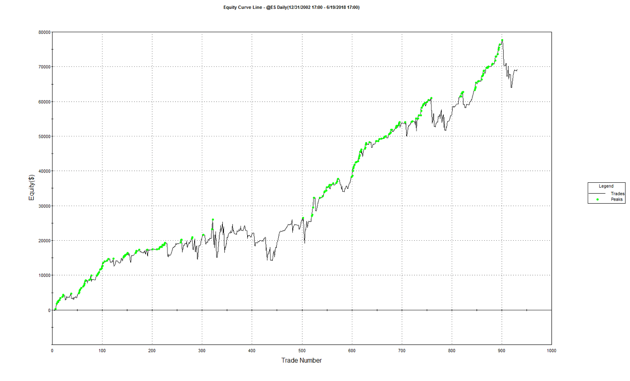
This is often as far as traders will take the idea, since it quickly gets a lot more complicated and challenging to build signals generated from an index series into the logic of a strategy designed for related, tradable market. And for that reason, there is a great deal of unexplored potential in using index data in this way. So, for instance, in the post below I discuss a swing trading system in the S&P500 E-mini futures (ticker: ES) that comprises several sub-systems build on prime-valued time intervals. This has the benefit of minimizing the overlap between signals from multiple sub-systems, thereby increasing temporal diversification.
A critical point about this system is that each of sub-systems trades the futures market based on data from both the E-mini contract and the S&P 500 cash index. A signal is generated when the system finds particular types of discrepancy between the cash index and corresponding futures, in a quasi risk-arbitrage.
Arbing the NASDAQ 100 Index Futures
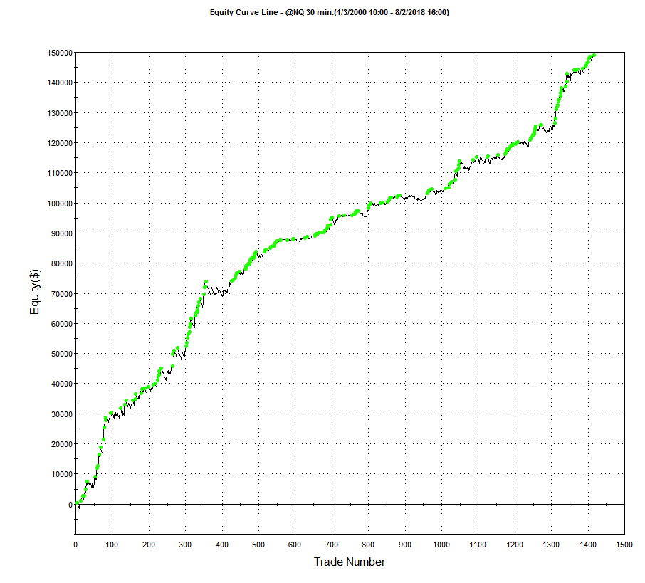
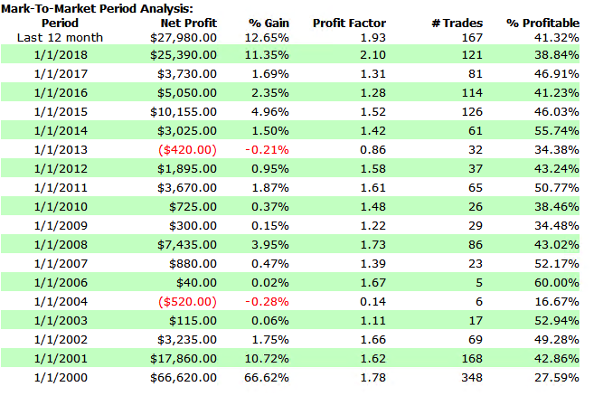
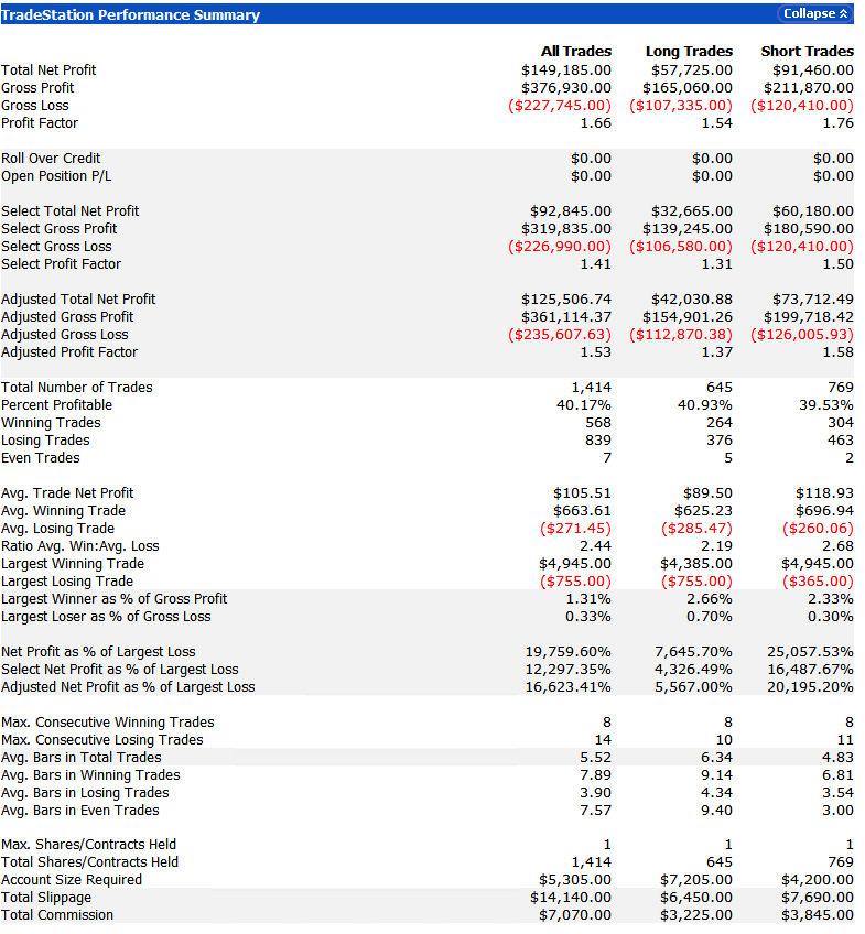
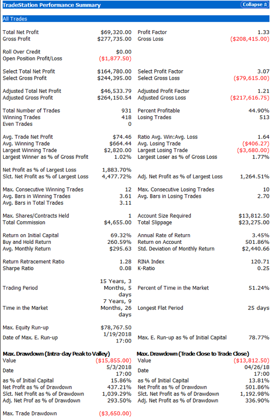
Developing trading systems for the S&P500 E-mini futures market is not that hard. A much tougher challenge, at least in my experience, is presented by the E-mini NASDAQ-100 futures (ticker: NQ). This is partly to do with the much smaller tick size and different market microstructure of the NASDAQ futures market. Additionally, the upward drift in equity related products typically favors strategies that are long-only. Where a system trades both long and short sides of the market, the performance on the latter is usually much inferior. This can mean that the strategy performs poorly in bear markets such as 2008/09 and, for the tech sector especially, the crash of 2000/2001. Our goal was to develop a daytrading system that might trade 1-2 times a week, and which would perform as well or better on short trades as on the long side. This is where NASDAQ 100 index data proved to be especially helpful. We found that discrepancies between the cash index and futures market gave particularly powerful signals when markets seemed likely to decline. Using this we were able to create a system that performed exceptionally well during the most challenging market conditions. It is notable that, in the performance results below (for a single futures contract, net of commissions and slippage), short trades contributed the greater proportion of total profits, with a higher overall profit factor and average trade size.
Conclusion: Using Index Data, Or Other Correlated Signals, Often Improves Performance
It is well worthwhile investigating how non-tradable index data can be used in a trading strategy, either as a qualifying signal or, more directly, within the logic of the algorithm itself. The greater challenge of building such systems means that there are opportunities to be found, even in well-mined areas like index futures markets. A parallel idea that likewise offers plentiful opportunity is in designing systems that make use of data on multiple time frames, and in correlated markets, for instance in the energy sector.Here one can identify situations in which, under certain conditions, one market has a tendency to lead another, a phenomenon referred to as Granger Causality.
Momentum trading strategies span a diverse range of trading ideas. Often they will use indicators to determine the recent underlying trend and try to gauge the strength of the trend using measures of the rate of change in the price of the asset.
One very simple momentum concept, a strategy in S&P500 E-Mini futures, is described in the following blog post:
The basic idea is to buy the S&P500 E-Mini futures when the contract makes a new intraday high. This is subject to the qualification that the Internal Bar Strength fall below a selected threshold level. In order words, after a period of short-term weakness – indicated by the low reading of the Internal Bar Strength – we buy when the futures recover to make a new intraday high, suggesting continued forward momentum.
IBS is quite a useful trading indicator, which you can learn more about in these posts:
I have developed a version of the intraday-high strategy, using parameters to generalize it and allow for strategy optimization. The Easylanguage code for my version of the strategy is as follows:
If H[IBSlag] > L[IBSlag] then
Begin
IBS=(H[IBSlag]-C[IBSlag])/(H[IBSlag]-L[IBSlag]);
end;
If (IBS <= IBStrigger) and (H[0] >= Highest(High, ndaysHigh)) then
begin
Buy nContracts contracts this bar on close;
end;
If C[0] > H[1] then
begin
Sell all contracts this bar on close;
end;
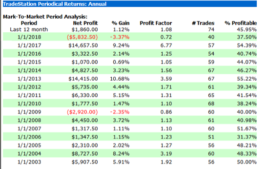
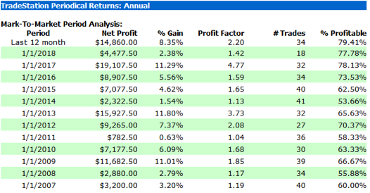
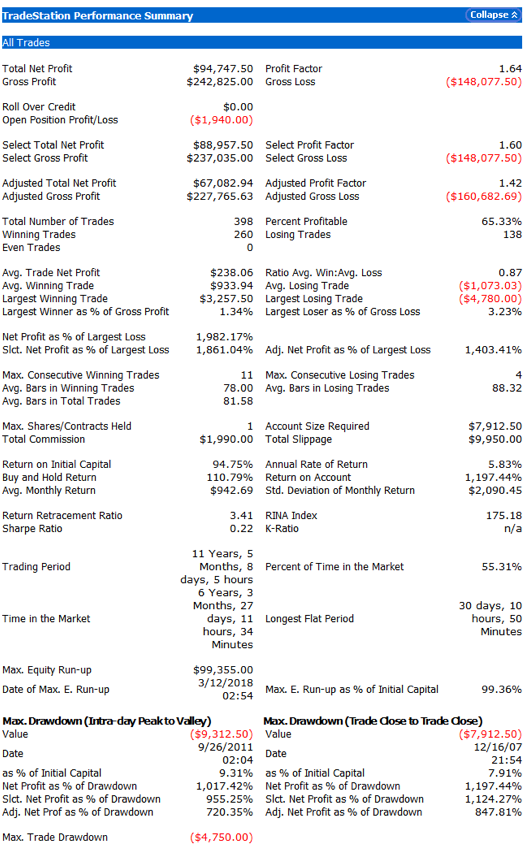
The performance results for the strategy appear quite promising, despite the downturn in strategy profitability in 2018 to date (all performance results are net of slippage and commission):
Robustness Testing with Walk Forward Optimization
We evaluate the robustness of the strategy using the Walk Forward Optimization feature in Tradestation. Walk forward analysis is the process of optimizing a trading system using a limited set of parameters, and then testing the best optimized parameter set on out-of-sample data. This process is similar to how a trader would use an automated trading system in real live trading. The in-sample time window is shifted forward by the period covered by the out-of-sample test, and the process is repeated. At the end of the test, all of the recorded results are used to assess the trading strategy.
In other words, walk forward analysis does optimization on a training set; tests on a period after the set and then rolls it all forward and repeats the process. This gives a larger out-of-sample period and allows the system developer to see how stable the system is over time.
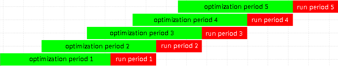
The image below illustrates the walk forward analysis procedure. An optimization is performed over a longer period (the in-sample data), and then the optimized parameter set is tested over a subsequent shorter period (the out-of-sample data). The optimization and testing periods are shifted forward, and the process is repeated until a suitable sample size is achieved.
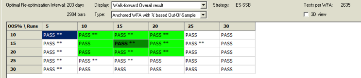
Tradestation enables the user to run a battery of WFO tests, using different size in-sample and out-of-sample sizes and number of runs. The outcome of each test is evaluated on several specific criteria such as the net profit and drawdown and only if the system meets all of the criteria is the test designated as a “Pass”. This gives the analyst a clear sense of the robustness of his strategy across multiple periods and sample sizes.
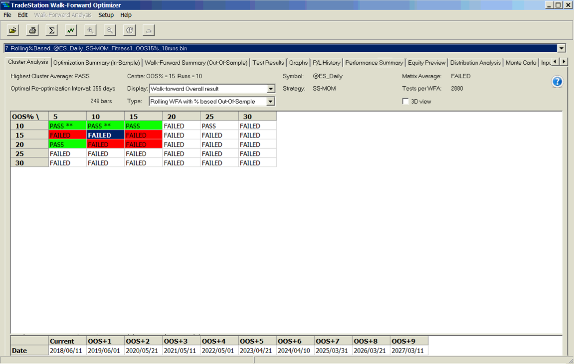
A WFO cluster analysis summary for the momentum strategy is illustrated below. The cluster test is designated as “Failed” overall, since the strategy failed to meet the test criteria for a preponderance of the individual walk-forward tests. The optimal parameters found in each test vary considerably over the sample periods spanning 2003-2018, giving concerns about the robustness of the strategy under changing market conditions.
Improving the Strategy
We can improve both the performance and robustness of our simple momentum strategy by combining it with several other trend and momentum indicators. One such example is illustrated in the performance charts and tables below. The strategy has performed well in both bull and bear markets and in both normal and volatile market conditions:
A WFO cluster analysis indicates that the revised momentum strategy is highly robust to the choice of sample size and strategy parameters, as it passes every test in the 30-cell WFO analysis cluster table:
Conclusion
Momentum strategies are well known and easy to develop using standard methodologies, such as the simple indicators used in this example. They tend to work well in most equity index futures markets, and in some commodity markets too. One of their big drawbacks, however, is that they typically go through periods of poor performance and need to be tested thoroughly for robustness in order to ensure satisfactory results under the full range of market conditions.
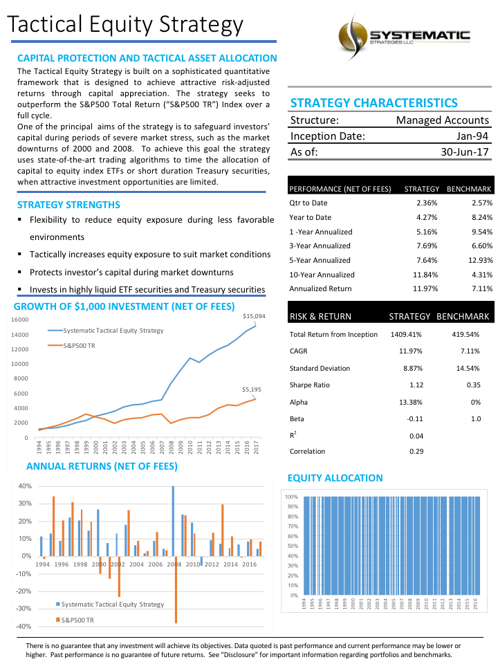
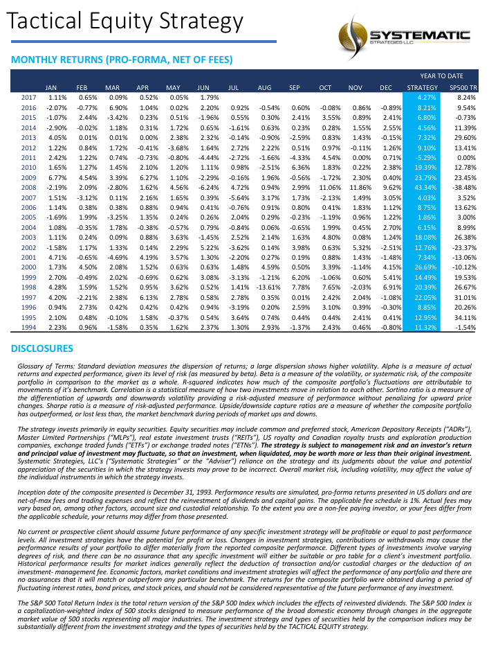
We have created a long-only equity strategy that aims to beat the S&P 500 total return benchmark by using tactical allocation algorithms to invest in equity ETFs. One of the principal goals of the strategy is to protect investors’ capital during periods of severe market stress such as in the downturns of 2000 and 2008. The strategy times the allocation of capital to equity ETFs or short-duration Treasury securities when investment opportunities are limited.
Systematic Strategies is a hedge fund rather than an RIA, so we have no plans to offer the product to the public. However, we are currently holding exploratory discussions with Registered Investment Advisors about how the strategy might be made available to their clients.
For more background, see this post on Seeking Alpha: http://tiny.cc/ba3kny
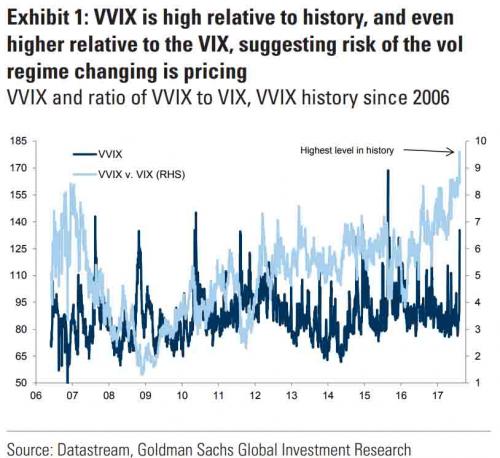
In a previous blog post I mentioned the VVIX/VIX Ratio, which is measured as the ratio of the CBOE VVIX Index to the VIX Index. The former measures the volatility of the VIX, or the volatility of volatility.
A follow-up article in ZeroHedge shortly afterwards pointed out that the VVIX/VIX ratio had reached record highs, prompting Goldman Sachs analyst Ian Wright to comment that this could signal the ending of the current low-volatility regime:
A linkedIn reader pointed out that individual stock volatility was currently quite high and when selling index volatility one is effectively selling stock correlations, which had now reached historically low levels. I concurred:
What’s driving the low vol regime is the exceptionally low level of cross-sectional correlations. And, as correlations tighten, index vol will rise. Worse, we are likely to see a feedback loop – higher vol leading to higher correlations, further accelerating the rise in index vol. So there is a second order, Gamma effect going on. We see that is the very high levels of the VVIX index, which shot up to 130 last week. The all-time high in the VVIX prior to Aug 2015 was around 120. The intra-day high in Aug 2015 reached 225. I’m guessing it will get back up there at some point, possibly this year.
As there appears to be some interest in the subject I decided to add a further blog post looking a little further into the relationship between volatility and correlation. To gain some additional insight we are going to make use of the CBOE implied correlation indices. The CBOE web site explains:
Using SPX options prices, together with the prices of options on the 50 largest stocks in the S&P 500 Index, the CBOE S&P 500 Implied Correlation Indexes offers insight into the relative cost of SPX options compared to the price of options on individual stocks that comprise the S&P 500.
CBOE calculates and disseminates two indexes tied to two different maturities, usually one year and two years out. The index values are published every 15 seconds throughout the trading day.
Both are measures of the expected average correlation of price returns of S&P 500 Index components, implied through SPX option prices and prices of single-stock options on the 50 largest components of the SPX.
Dispersion Trading
One application is dispersion trading, which the CBOE site does a good job of summarizing:
The CBOE S&P 500 Implied Correlation Indexes may be used to provide trading signals for a strategy known as volatility dispersion (or correlation) trading. For example, a long volatility dispersion trade is characterized by selling at-the-money index option straddles and purchasing at-the-money straddles in options on index components. One interpretation of this strategy is that when implied correlation is high, index option premiums are rich relative to single-stock options. Therefore, it may be profitable to sell the rich index options and buy the relatively inexpensive equity options.
The VIX Index and the Implied Correlation Indices
Again, the CBOE web site is worth quoting:
The CBOE S&P 500 Implied Correlation Indexes measure changes in the relative premium between index options and single-stock options. A single stock’s volatility level is driven by factors that are different from what drives the volatility of an Index (which is a basket of stocks). The implied volatility of a single-stock option simply reflects the market’s expectation of the future volatility of that stock’s price returns. Similarly, the implied volatility of an index option reflects the market’s expectation of the future volatility of that index’s price returns. However, index volatility is driven by a combination of two factors: the individual volatilities of index components and the correlation of index component price returns.
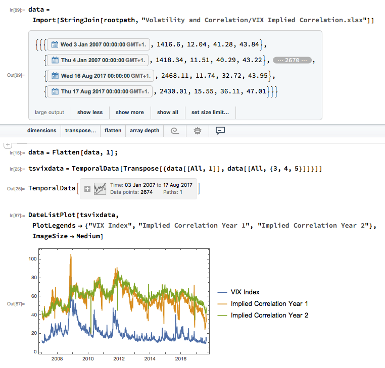
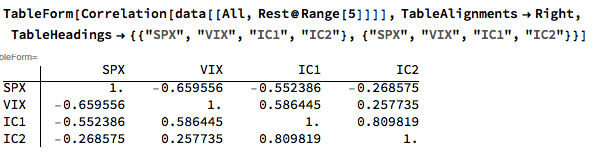
Let’s dig into this analytically. We first download and plot the daily for the VIX and Correlation Indices from the CBOE web site, from which it is evident that all three series are highly correlated:
An inspection reveals significant correlations between the VIX index and the two implied correlation indices, which are themselves highly correlated. The S&P 500 Index is, of course, negatively correlated with all three indices:
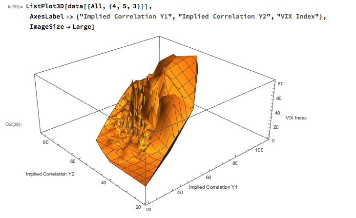
Modeling Volatility-Correlation
The response surface that describes the relationship between the VIX index and the two implied correlation indices is locally very irregular, but the slope of the surface is generally positive, as we would expect, since the level of VIX correlates positively with that of the two correlation indices.
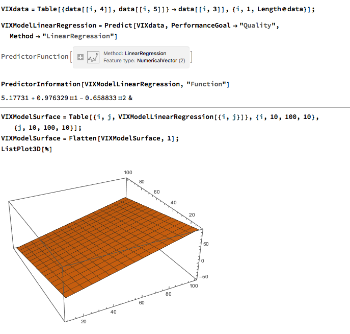
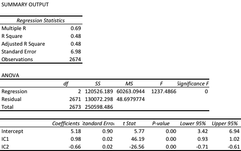
The most straightforward approach is to use a simple linear regression specification to model the VIX level as a function of the two correlation indices. We create a VIX Model Surface object using this specification with the Mathematica Predict function:The linear model does quite a good job of capturing the positive gradient of the response surface, and in fact has a considerable amount of explanatory power, accounting for a little under half the variance in the level of the VIX index:
However, there are limitations. To begin with, the assumption of independence between the explanatory variables, the correlation indices, clearly does not hold. In cases such as this, where explanatory variables are multicolinear, we are unable to draw inferences about the explanatory power of individual regressors, even though the model as a whole may be highly statistically significant, as here.
Secondly, a linear regression model is not going to capture non-linearities in the volatility-correlation relationship that are evident in the surface plot. This is confirmed by a comparison plot, which shows that the regression model underestimates the VIX level for both low and high values of the index:
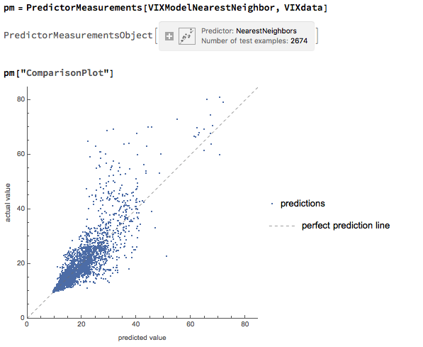
We can achieve a better outcome using a machine learning algorithm such as nearest neighbor, which is able to account for non-linearities in the response surface:
The comparison plot shows a much closer correspondence between actual and predicted values of the VIX index, even though there is evidence of some remaining heteroscedasticity in the model residuals:
Conclusion
A useful way to think about index volatility is as a two dimensional process, with time-series volatility measured on one dimension and dispersion (cross-sectional volatility, the inverse of correlation) measured on the second. The two factors are correlated and, as we have shown here, interact in a complicated, non-linear way.
The low levels of index volatility we have seen in recent months result, not from low levels of volatility in component stocks, but in the historically low levels of correlation (high levels of dispersion) in the underlying stock returns processes. As correlations begin to revert to historical averages, the impact will be felt in an upsurge in index volatility, compounded by the non-linear interaction between the two factors.
Recently I have been discussing possible areas of collaboration with an RIA contact on LinkedIn, who also happens to be very familiar with the hedge fund world. He outlined the case of a high net worth investor in equities (long only), who wanted to remain invested, but was becoming increasingly concerned about the prospects for a significant market downturn, or even a market crash, similar to those of 2000 or 2008.
I am guessing he is not alone: hardly a day goes by without the publication of yet another article sounding a warning about stretched equity valuations and the dangerously elevated level of the market.
The question put to me was, what could be done to reduce the risk in the investor’s portfolio?
Typically, conservative investors would have simply moved more of their investment portfolio into fixed income securities, but with yields at such low levels this is hardly an attractive option today. Besides, many see the bond market as representing an even more extreme bubble than equities currently.
Hedging Strategies
The problem with traditional hedging mechanisms such as put options, for example, is that they are relatively expensive and can easily reduce annual returns from the overall portfolio by several hundred basis points. Even at current low level of volatility the performance drag is noticeable, since the potential upside in the equity portfolio is also lower than it has been for some time. A further consideration is that many investors are not mandated – or are simply reluctant – to move beyond traditional equity investing into complex ETF products or derivatives.
An equity long/short hedge fund product is one possible solution, but many equity investors are reluctant to consider shorting stocks under any circumstances, even for hedging purposes. And while a short hedge may provide some downside protection it is unlikely to fully safeguard the investor in a crash scenario. Furthermore, the cost of a hedge fund investment is typically greater than for a long-only product, entailing the payment of a performance fee in addition to management fees that are often higher than for standard investment products.
The Ideal Investment Strategy
Given this background, we can say that the ideal investment strategy is one that:
Invests long-only in equities
Is inexpensive to implement (reasonable management fees; no performance fees)
Does not require shorting stocks, or expensive hedging mechanisms such as options
Makes acceptable returns during both bull and bear markets
Is likely to produce positive returns in a market crash scenario
A typical buy-and-hold approach is unlikely to meet only the first three requirements, although an argument could be made that a judicious choice of defensive stocks might enable the investment portfolio to generate returns at an “acceptable” level during a downturn (without being prescriptive as to the precise meaning of that term may be). But no buy-and-hold strategy could ever be expected to prosper during times of severe market stress. A more sophisticated approach is required.
Market Timing
Market timing is regarded as a “holy grail” by some quantitative strategists. The idea, simply, is to increase or reduce risk exposure according to the prospects for the overall market. For a very long time the concept has been dismissed as impossible, by definition, given that markets are mostly efficient. But analysts have persisted in the attempt to develop market timing techniques, motivated by the enormous benefits that a viable market timing strategy would bring. And gradually, over time, evidence has accumulated that the market can be timed successfully and profitably. The rate of progress has accelerated in the last decade by the considerable advances in computing power and the development of machine learning algorithms and application of artificial intelligence to investment finance.
I have written several articles on the subject of market timing that the reader might be interested to review (see below). In this article, however, I want to focus firstly on the work on another investment strategist, Blair Hull.
Blair Hull rose to prominence in the 1980’s and 1990’s as the founder of the highly successful quantitative option market making firm, the Hull Trading Company which at one time moved nearly a quarter of the entire daily market volume on some markets, and executed over 7% of the index options traded in the US. The firm was sold to Goldman Sachs at the peak of the equity market in 1999, for a staggering $531 million.
Blair used the capital to establish the Hull family office, Hull Investments, and in 2013 founded an RIA, Hull Tactical Asset Allocation LLC. The firm’s investment thesis is firmly grounded in the theory of market timing, as described in the paper “A Practitioner’s Defense of Return Predictability”, authored by Blair Hull and Xiao Qiao, in which the issues and opportunities of market timing and return predictability are explored.
In 2015 the firm launched The Hull Tactical Fund (NYSE Arca: HTUS), an actively managed ETF that uses quantitative trading model to take long and short positions in ETFs that seek to track the performance of the S&P 500, as well as leveraged ETFs or inverse ETFs that seek to deliver multiples, or the inverse, of the performance of the S&P 500. The goal to achieve long-term growth from investments in the U.S. equity and Treasury markets, independent of market direction.
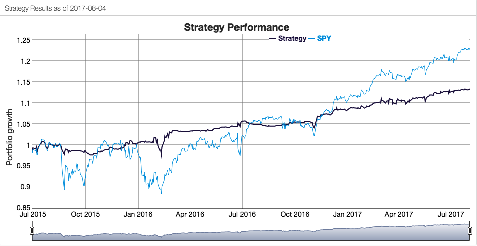
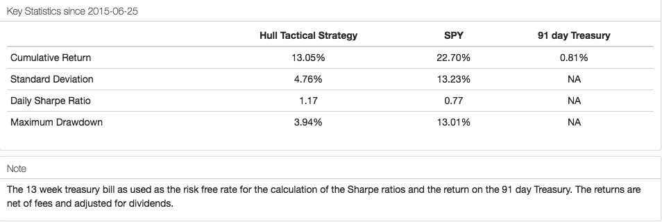
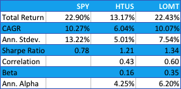
How well has the Hull Tactical strategy performed? Since the fund takes the form of an ETF its performance is a matter in the public domain and is published on the firm’s web site. I reproduce the results here, which compare the performance of the HTUS ETF relative to the SPDR S&P 500 ETF (NYSE Arca: SPY):
Although the HTUS ETF has underperformed the benchmark SPY ETF since launching in 2015, it has produced a higher rate of return on a risk-adjusted basis, with a Sharpe ratio of 1.17 vs only 0.77 for SPY, as well as a lower drawdown (-3.94% vs. -13.01%). This means that for the same “risk budget” as required to buy and hold SPY, (i.e. an annual volatility of 13.23%), the investor could have achieved a total return of around 36% by using margin funds to leverage his investment in HTUS by a factor of 2.8x.
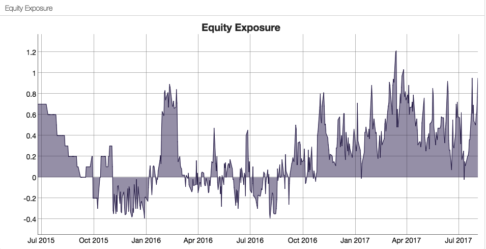
How does the Hull Tactical team achieve these results? While the detailed specifics are proprietary, we know from the background description that market timing (and machine learning concepts) are central to the strategy and this is confirmed by the dynamic level of the fund’s equity exposure over time:
A Long-Only, Crash-Resistant Equity Strategy
A couple of years ago I and my colleagues carried out an investigation of long-only equity strategies as part of a research project. Our primary focus was on index replication, but in the course of our research we came up with a methodology for developing long-only strategies that are highly crash-resistant.
The performance of our Long-Only Market Timing strategy is summarized below and compared with the performance of the HTUS ETF and benchmark SPY ETF (all results are net of fees). Over the period from inception of the HTUS ETF, our LOMT strategy produced a higher total return than HTUS (22.43% vs. 13.17%), higher CAGR (10.07% vs. 6.04%), higher risk adjusted returns (Sharpe Ratio 1.34 vs 1.21) and larger annual alpha (6.20% vs 4.25%). In broad terms, over this period the LOMT strategy produced approximately the same overall return as the benchmark SPY ETF, but with a little over half the annual volatility.
Application of Artificial Intelligence to Market Timing
Like the HTUS ETF, our LOMT strategy operates with very low fees, comparable to an ETF product rather than a hedge fund (1% management fee, no performance fees). Again, like the HTUS ETF our LOMT products makes no use of leverage. However, unlike HTUS it avoids complicated (and expensive) inverse or leveraged ETF products and instead invests only in two assets – the SPY ETF and 91-day US Treasury Bills. In other words, the LOMT strategy is a pure market timing strategy, moving capital between the SPY ETF and Treasury Bills depending on its forecast of future market performance. These forecasts are derived from machine learning algorithms that are specifically tuned to minimize the downside risk in the investment portfolio. This not only makes strategy returns less volatile, but also ensures that the strategy is very robust to market downturns.
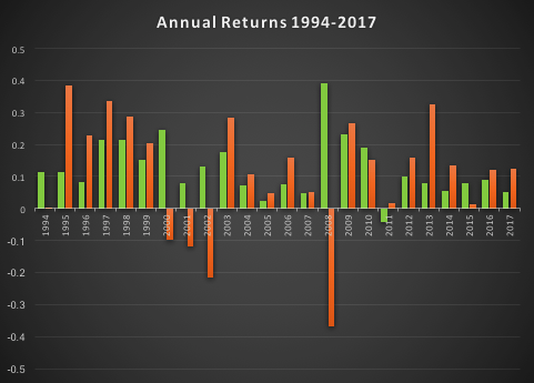
In fact, even better than that, not only does the LOMT strategy tend to avoid large losses during periods of market stress, it is capable of capitalizing on the opportunities that more volatile market conditions offer. Looking at the compounded returns (net of fees) over the period from 1994 (the inception of the SPY ETF) we see that the LOMT strategy produces almost double the total profit of the SPY ETF, despite several years in which it underperforms the benchmark. The reason is clear from the charts: during the periods 2000-2002 and again in 2008, when the market crashed and returns in the SPY ETF were substantially negative, the LOMT strategy managed to produce positive returns. In fact, the banking crisis of 2008 provided an exceptional opportunity for the LOMT strategy, which in that year managed to produce a return nearing +40% at a time when the SPY ETF fell by almost the same amount!
Long Volatility Strategies
I recall having a conversation with Nassim Taleb, of Black Swan fame, about his Empirica fund around the time of its launch in the early 2000’s. He explained that his analysis had shown that volatility was often underpriced due to an under-estimation of tail risk, which the fund would seek to exploit by purchasing cheap out-of-the-money options. My response was that this struck me a great idea for an insurance product, but not a hedge fund – his investors, I explained, were going to hate seeing month after month of negative returns and would flee the fund. By the time the big event occurred there wouldn’t be sufficient AUM remaining to make up the shortfall. And so it proved.
A similar problem arises from most long-volatility strategies, whether constructed using options, futures or volatility ETFs: the combination of premium decay and/or negative carry typically produces continuing losses that are very difficult for the investor to endure.
Conclusion
What investors have been seeking is a strategy that can yield positive returns during normal market conditions while at the same time offering protection against the kind of market gyrations that typically decimate several years of returns from investment portfolios, such as we saw after the market crashes in 2000 and 2008. With the new breed of long-only strategies now being developed using machine learning algorithms, it appears that investors finally have an opportunity to get what they always wanted, at a reasonable price.
And just in time, if the prognostications of the doom-mongers turn out to be correct.