
Strategy Portfolio Construction

Applications of Graph Theory In Finance
Analyzing Big Data
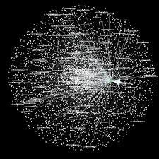
Very large datasets – comprising voluminous numbers of symbols – present challenges for the analyst, not least of which is the difficulty of visualizing relationships between the individual component assets. Absent the visual clues that are often highlighted by graphical images, it is easy for the analyst to overlook important changes in relationships. One means of tackling the problem is with the use of graph theory.

DOW 30 Index Member Stocks Correlation Graph
In this example I have selected a universe of the Dow 30 stocks, together with a sample of commodities and bonds and compiled a database of daily returns over the period from Jan 2012 to Dec 2013. If we want to look at how the assets are correlated, one way is to created an adjacency graph that maps the interrelations between assets that are correlated at some specified level (0.5 of higher, in this illustration).
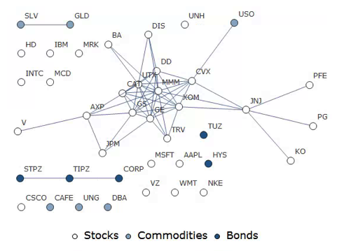
Obviously the choice of correlation threshold is somewhat arbitrary, and it is easy to evaluate the results dynamically, across a wide range of different threshold parameters, say in the range from 0.3 to 0.75:

The choice of parameter (and time frame) may be dependent on the purpose of the analysis: to construct a portfolio we might select a lower threshold value; but if the purpose is to identify pairs for possible statistical arbitrage strategies, one will typically be looking for much higher levels of correlation.
Correlated Cliques
Reverting to the original graph, there is a core group of highly inter-correlated stocks that we can easily identify more clearly using the Mathematica function FindClique to specify graph nodes that have multiple connections:
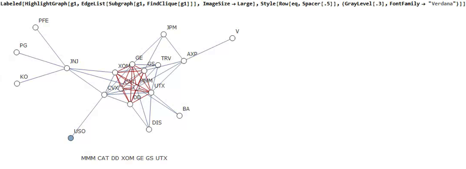
We might, for example, explore the relative performance of members of this sub-group over time and perhaps investigate the question as to whether relative out-performance or under-performance is likely to persist, or, given the correlation characteristics of this group, reverse over time to give a mean-reversion effect.
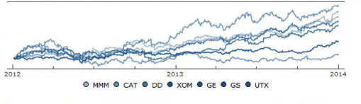
Constructing a Replicating Portfolio
An obvious application might be to construct a replicating portfolio comprising this equally-weighted sub-group of stocks, and explore how well it tracks the Dow index over time (here I am using the DIA ETF as a proxy for the index, for the sake of convenience):
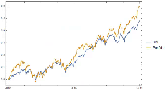
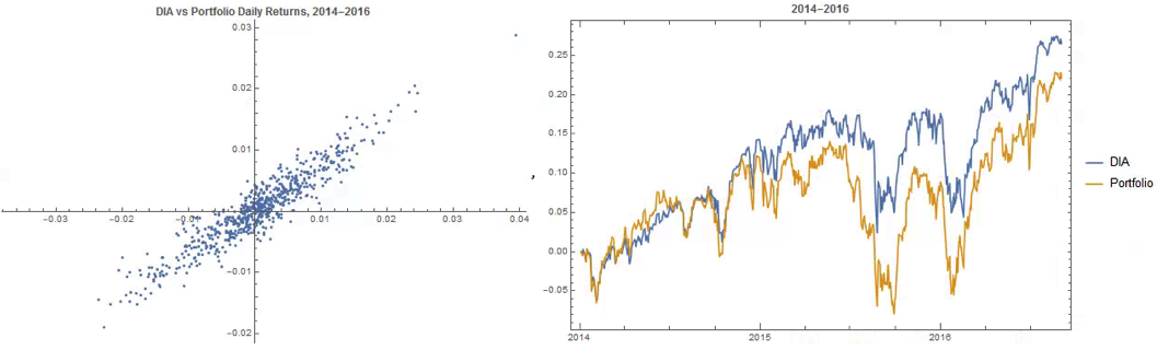
The correlation between the Dow index (DIA ETF) and the portfolio remains strong (around 0.91) throughout the out-of-sample period from 2014-2016, although the performance of the portfolio is distinctly weaker than that of the index ETF after the early part of 2014:
Constructing Robust Portfolios
Another application might be to construct robust portfolios of lower-correlated assets. Here for example we use the graph to identify independent vertices that have very few correlated relationships (designated using the star symbol in the graph below). We can then create an equally weighted portfolio comprising the assets with the lowest correlations and compare its performance against that of the Dow Index.
The new portfolio underperforms the index during 2014, but with lower volatility and average drawdown.

Conclusion – Graph Theory has Applications in Portfolio Constructions and Index Replication
Graph theory clearly has a great many potential applications in finance. It is especially useful as a means of providing a graphical summary of data sets involving a large number of complex interrelationships, which is at the heart of portfolio theory and index replication. Another useful application would be to identify and evaluate correlation and cointegration relationships between pairs or small portfolios of stocks, as they evolve over time, in the context of statistical arbitrage.
The Correlation Signal

The use of correlations is widespread in investment management theory and practice, from the construction of portfolios to the design of hedge trades to statistical arbitrage strategies.
A common difficulty encountered in all of these applications is the variation in correlation: assets that at one time appear to be suitably uncorrelated for hedging purposes, may become much more highly correlated at other times, such as periods of market stress. Conversely, stocks that appear suitable for pairs trading due to the high correlation in their prices or returns, may de-couple at a later time, causing significant losses.
The instability in the level of correlation is further aggravated by the empirical finding that the volatility in correlation is itself time-dependent: at times the correlations between assets may appear to fluctuate smoothly within a tight range; at other times we might see several fluctuations in the sign of the correlation coefficient over the course of a few days.
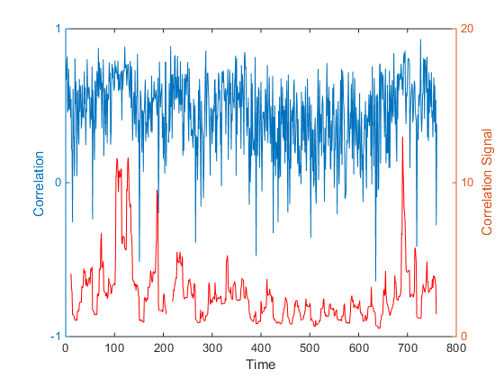
One tool I have found useful in this context is a concept I refer to as the correlation signal, defined at the average correlation divided by the standard deviation of the correlation coefficient. The chart below illustrates a typical pattern for a pair of Oil and Gas industry stocks. The blue line is the average daily correlation between the stocks, measured at 5-minute intervals. The red line is the correlation signal – the average daily correlation divided by the standard deviation in the intra-day correlation. The stochastic nature of both the correlation coefficient and the correlation signal is quite evident. Note that the correlation signal, unlike the coefficient, is not constrained within the limits of +/- 1. At times when the variation in correlation is low the signal an easily exceed those limits by as much as an order of magnitude.
In later posts I will illustrate the usefulness of the correlation signal in portfolio construction and statistical arbitrage. For now, let me just say that it is a measure of the strength of the correlation as a signal, relative to the noise of random variation in the correlation process. It can be used to identify situations in which a relationship – whether a positive or negative correlation – appears to be stable or unstable, and therefore viable as a basis for inference, or not.