Pairs Trading = Numbers Game
One of the first things you quickly come to understand in equity pairs trading is how important it is to spread your risk. The reason is obvious: stocks are subject to a multitude of risk factors – amongst them earning shocks and corporate actions -that can blow up an otherwise profitable pairs trade. Instead of the pair re-converging, they continue to diverge until you are stopped out of the position. There is not much you can do about this, because equities are inherently risky. Some arbitrageurs prefer trading ETF pairs for precisely this reason. But risk and reward are two sides of the same coin: risks tend to be lower in ETF pairs trades, but so, too, are the rewards. Another factor to consider is that there are many more opportunities to be found amongst the vast number of stock combinations than in the much smaller universe of ETFs. So equities remain the preferred asset class of choice for the great majority of arbitrageurs.
 So, because of the risk in trading equities, it is vitally important to spread the risk amongst a large number of pairs. That way, when one of your pairs trades inevitably blows up for one reason or another, the capital allocation is low enough not to cause irreparable damage to the overall portfolio. Nor are you over-reliant on one or two star performers that may cease to contribute if, for example, one of the stock pairs is subject to a merger or takeover.
Does that mean that pairs trading is accessible only to managers with deep enough pockets to allocate broadly in the investment universe? Yes and no. On the one hand, of course, you need sufficient capital to allocate a meaningful sum to each of your pairs. But pairs trading is highly efficient in its use of capital: margin requirements are greatly reduced by the much lower risk of a dollar-neutral portfolio. So your capital goes further than in would in a long-only strategy, for example.
How many pair combinations would you need to research to build an investment portfolio of the required size? The answer might shock you: millions. Or even tens of millions. In the case of the Gemini Pairs strategy, for example, the universe comprises around 10m stock pairs and 200,000 ETF combinations.
It turns out to be much more challenging to find reliable stock pairs to trade than one might imagine, for reasons I am about to discuss. So what tends to discourage investors from exploring pairs trading as an investment strategy is not because the strategy is inherently hard to understand; nor because the methods are unknown; nor because it requires vast amounts of investment capital to be viable. It is that the research effort required to build a successful statistical arbitrage strategy is beyond the capability of the great majority of investors.
Before you become too discouraged, I will just say that there are at least two solutions to this challenge I can offer, which I will discuss later.
Methodology Isn’t a Decider
I have traded pairs successfully using all of the techniques described in the first part of the post (i.e. Ratio, Regression, Kalman and Copula methods). Equally, I have seen a great many failed pairs strategies produced by using every available technique. There is no silver bullet. One often finds that a pair that perform poorly using the ratio method produces decent returns when a regression or Kalman Filter model is applied. From experience, there is no pattern that allows you to discern which technique, if any, is gong to work. You have to be prepared to try all of them, at least in back-test.
Correlation is Not the Answer
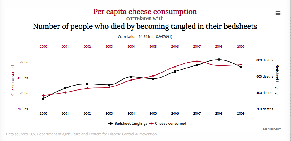
In a typical description of pairs trading the first order of business is often to look for a highly correlated pairs to trade. While this makes sense as a starting point, it can never provide a complete answer. The reason is well known: correlations are unstable, and can often arise from random chance rather than as a result of a real connection between two stock processes. The concept of spurious correlation is most easily grasped with an example, for instance:
Of course, no rational person believes that there is a causal connection between cheese consumption and death by bedsheet entanglement – it is a spurious correlation that has arisen due to the random fluctuations in the two time series. And because the correlation is spurious, the apparent relationship is likely to break down in future.
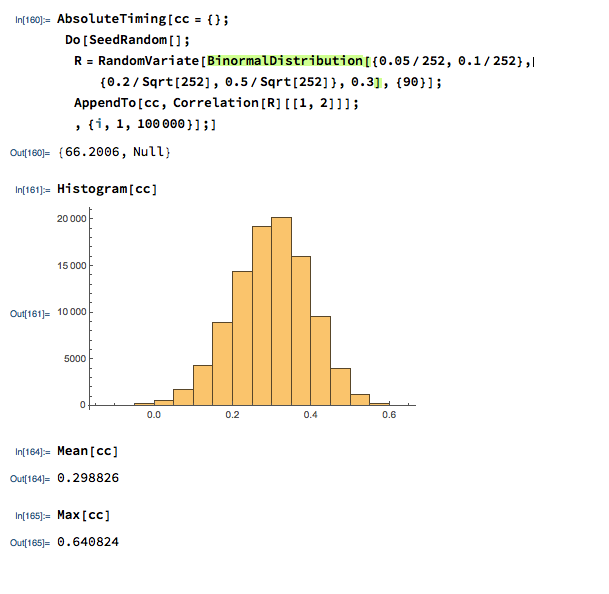
We can provide a slightly more realistic illustration as follows. Let us suppose we have two correlated stocks, one with annual drift (i.e trend of 5% and annual volatility of 25%, the other with annual drift of 20% and annual volatility of 50%. We assume that returns from the two processes follow a Normal distribution, with true correlation of 0.3. Let’s assume that we sample the returns for the two stocks over 90 days to estimate the correlation, simulating the real-world situation in which the true correlation is unknown. Unlike in the real-world scenario, we can sample the 90-day returns many times (100,000 in this experiment) and look at the range of correlation estimates we observe:
We find that, over the 100,000 repeated experiments the average correlation estimate is very close indeed to the true correlation. However, in the real-world situation we only have a single observation, based on the returns from the two stock processes over the prior 90 days. If we are very lucky, we might happen to pick a period in which the processes correlate at a level close to the true value of 0.3. But as the experiment shows, we might be unlucky enough to see an estimate as high as 0.64, or as low as zero!
So when we look at historical data and use estimates of the correlation coefficient to gauge the strength of the relationship between two stocks, we are at the mercy of random variation in the sampling process, one that could suggest a much stronger (or weaker) connection than is actually the case.
One is on firmer ground in selecting pairs of stocks in the same sector, for example oil or gold-mining stocks, because we are able to identify causal factors that should provide a basis for a reliable correlation, such as the price of oil or gold. This is indeed one of the “screens” that statistical arbitrageurs often use to select pairs for analysis. But there are many examples of stocks that “ought” to be correlated but which nonetheless break down and drift apart. This can happen for many reasons: changes in the capital structure of one of the companies; a major product launch; regulatory action; or corporate actions such as mergers and takeovers.
The bottom line is that correlation, while important, is not by itself a sufficiently reliable measure to provide a basis for pair selection.
Cointegration: the Drunk and His Dog
Suppose you see two drunks (i.e., two random walks) wandering around. The drunks don’t know each other (they’re independent), so there’s no meaningful relationship between their paths.
But suppose instead you have a drunk walking with his dog. This time there is a connection. What’s the nature of this connection? Notice that although each path individually is still an unpredictable random walk, given the location of one of the drunk or dog, we have a pretty good idea of where the other is; that is, the distance between the two is fairly predictable. (For example, if the dog wanders too far away from his owner, he’ll tend to move in his direction to avoid losing him, so the two stay close together despite a tendency to wander around on their own.) We describe this relationship by saying that the drunk and her dog form a cointegrating pair.
In more technical terms, if we have two non-stationary time series X and Y that become stationary when differenced (these are called integrated of order one series, or I(1) series; random walks are one example) such that some linear combination of X and Y is stationary (aka, I(0)), then we say that X and Y are cointegrated. In other words, while neither X nor Y alone hovers around a constant value, some combination of them does, so we can think of cointegration as describing a particular kind of long-run equilibrium relationship. (The definition of cointegration can be extended to multiple time series, with higher orders of integration.)
Other examples of cointegrated pairs:
- Income and consumption: as income increases/decreases, so too does consumption.
- Size of police force and amount of criminal activity
- A book and its movie adaptation: while the book and the movie may differ in small details, the overall plot will remain the same.
- Number of patients entering or leaving a hospital
So why do we care about cointegration? Someone else can probably give more econometric applications, but in quantitative finance, cointegration forms the basis of the pairs trading strategy: suppose we have two cointegrated stocks X and Y, with the particular (for concreteness) cointegrating relationship X – 2Y = Z, where Z is a stationary series of zero mean. For example, X could be McDonald’s, Y could be Burger King, and the cointegration relationship would mean that X tends to be priced twice as high as Y, so that when X is more than twice the price of Y, we expect X to move down or Y to move up in the near future (and analogously, if X is less than twice the price of Y, we expect X to move up or Y to move down). This suggests the following trading strategy: if X – 2Y > d, for some positive threshold d, then we should sell X and buy Y (since we expect X to decrease in price and Y to increase), and similarly, if X – 2Y < -d, then we should buy X and sell Y.
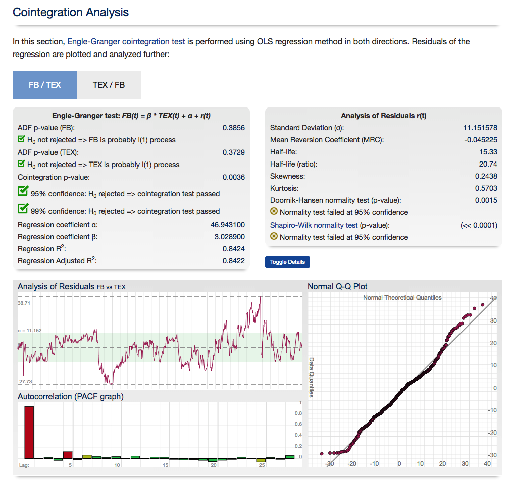
So how do you detect cointegration? There are several different methods, but the simplest is probably the Engle-Granger test, which works roughly as follows:
- Check that Xt and Yt are both I(1).
- Estimate the cointegrating relationship =+Yt=aXt+et by ordinary least squares.
- Check that the cointegrating residuals et are stationary (say, by using a so-called unit root test, e.g., the Dickey-Fuller test).
Also, something else that should perhaps be mentioned is the relationship between cointegration and error-correction mechanisms: suppose we have two cointegrated series ,Xt,Yt, with autoregressive representations
=−1+−1+Xt=aXt−1+bYt−1+ut
=−1+−1+Yt=cXt−1+dYt−1+vt
By the Granger representation theorem (which is actually a bit more general than this), we then have
Δ=1(−1−−1)+ΔXt=α1(Yt−1−βXt−1)+ut
Δ=2(−1−−1)+ΔYt=α2(Yt−1−βXt−1)+vt
where −1−−1∼(0)Yt−1−βXt−1∼I(0) is the cointegrating relationship. Regarding −1−−1Yt−1−βXt−1 as the extent of disequilibrium from the long-run relationship, and the αi as the speed (and direction) at which the time series correct themselves from this disequilibrium, we can see that this formalizes the way cointegrated variables adjust to match their long-run equilibrium.
So, just to summarize a bit, cointegration is an equilibrium relationship between time series that individually aren’t in equilibrium (you can kind of contrast this with (Pearson) correlation, which describes a linear relationship), and it’s useful because it allows us to incorporate both short-term dynamics (deviations from equilibrium) and long-run expectations , i.e. corrections to equilibrium. (My thanks to Edwin Chen for this entertaining explanation)
Cointegration is Not the Answer
So a typical workflow for researching possible pairs trade might be to examine a large number of pairs in a sector of interest, select those that meet some correlation threshold (e.e. 90%), test those pairs for cointegration and select those that appear to be cointegrated. The problem is: it doesn’t work! The pairs thrown up by this process are likely to work for a while, but many (even the majority) will break down at some point, typically soon after you begin live trading. `The reason is that all of the major statistical tests for cointegration have relatively low power and pairs that are apparently cointegrated break down suddenly, with consequential losses for the trader. The following posts delves into the subject in some detail:
Other Practical “Gotchas”
Apart from correlations/cointegration breakdowns there is a long list of things that can go wrong with a pairs trade that the practitioner needs to take account of, for instance:
- A stock may become difficult or expensive to short
- The overall backtest performance stats for a pair may look great, but the P&L per share is too small to overcome trading costs and other frictions.
- Corporate actions (mergers, takeovers) and earnings can blow up one side of an otherwise profitable pair.
- It is possible to trade passively, crossing the spread to trade the other leg when the first leg trades. But this trade expression is challenging to test. If paying the spread on both legs is going to jeopardize the profitability of the strategy, it is probably better to reject the pair.
What Works
From my experience, the testing phase of the process of building a statistical arbitrage strategy is absolutely critical. By this I mean that, after screening for correlation and cointegration, and back-testing all of the possible types of model, it is essential to conduct an extensive simulation test over a period of several weeks before adding a new pair to the production system. Testing is important for any algorithmic strategy, of course, but it is an integral part of the selection process where pairs trading is concerned. You should expect 60% to 80% of your candidates to fail in simulated trading, even after they have been carefully selected and thoroughly back-tested. The good good news is that those pairs that pass the final stage of testing usually are successful in a production setting.
Implementation
Putting all of this information together, it should be apparent that the major challenge in pairs trading lies not so much in understanding and implementing methodologies and techniques, but in implementing the research process on an industrial scale, sufficient to collate and analyze tens of millions of pairs. This is beyond the reach of most retail investors, and indeed, many small trading firms: I once worked with a trading firm for over a year on a similar research project, but in the end it proved to be capabilities of even their highly competent development team.
So does this mean that for the average quantitative strategist investors statistical arbitrage must remain an investment concept of purely theoretical interest? Actually, no. Firstly, for the investor, there are plenty of investment products available that they can access via hedge fund structures (or even our algotrading platform, as I have previously mentioned).
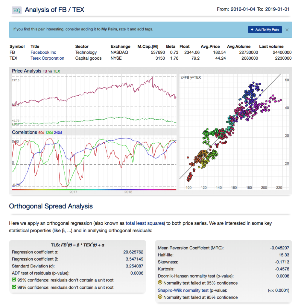
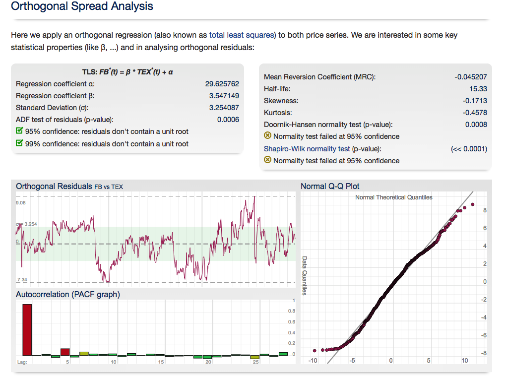
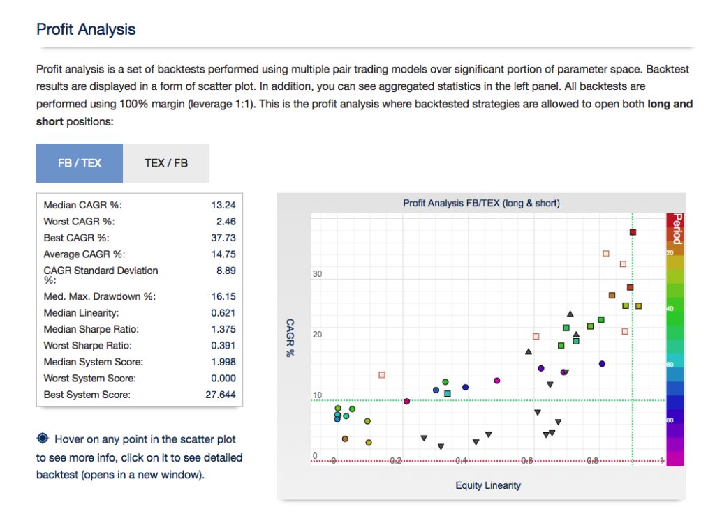
For those interested in building stat arb strategies there is an excellent resource that collates all of the data and analysis on tens of millions of stock pairs that enables the researcher to identify promising pairs, test their level of cointegration, backtest strategies using different methodologies and even put selected pars strategies into production (see example below).
Those interested should contact me for more information.

