Dynamic Time Warping


QUANTITATIVE RESEARCH AND TRADING
The latest theories, models and investment strategies in quantitative research and trading

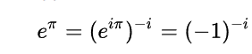
One of the most beautiful equations in the whole of mathematics is the identity (and its derivation):
I recently came across another beautiful mathematical concept that likewise relates the two transcendental numbers e and Pi.
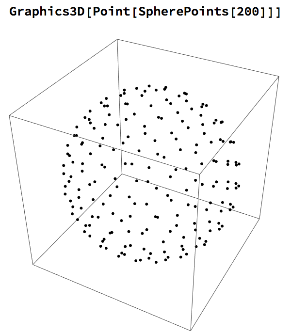
We begin by reviewing the concept of a unit sphere, which in 3-dimensional space is the region of points described by the equation:
![]()
We can some generate random coordinates that satisfy the equation, to produce the expected result:
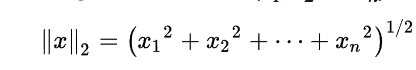
The equation above represents a 3-D unit sphere using the standard Euclidean Norm. It can be generalized to produce a similar formula for an n-dimensional hyper-sphere:
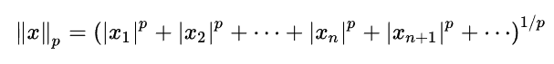
Another way to generalize the concept is by extending the Euclidean distance measure with what are referred to as p-Norms, or L-p spaces:
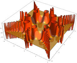
The shape of a unit sphere in L-p space can take many different forms, including some that have “corners”. Here are some examples of 2-dimensional spheres for values of p varying in the range { 0.25, 4}:
which can also be explored in the complex plane:
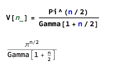
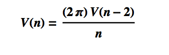
Reverting to the regular Euclidean metric, let’s focus on the n-dimensional unit hypersphere, whose volume is given by:
To see this, note that the volume of the unit sphere in 2-D space is just the surface area of a unit circle, which has area V(2) = π. Furthermore:
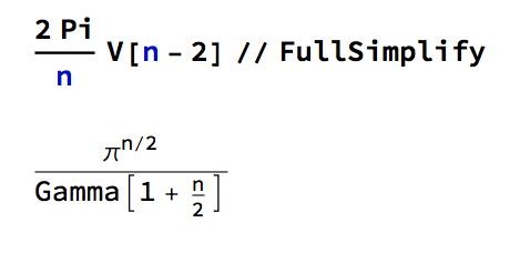
This is the equation for the volume of the unit hypersphere in n dimensions. Hence we have the following recurrence relationship:
 This recursion allows us to prove the equation for the volume of the unit hypersphere, by induction.
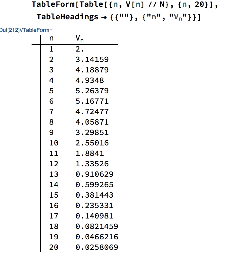
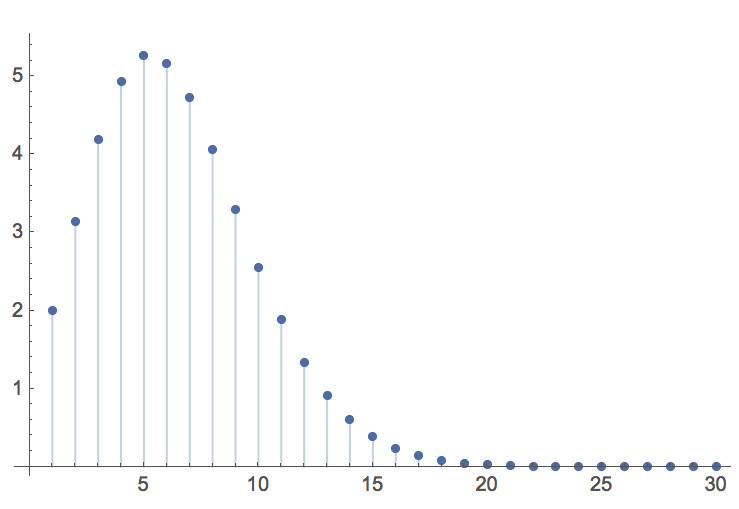
The function V(n) take a maximal value of 5.26 for n = 5 dimensions, thereafter declining rapidly towards zero:
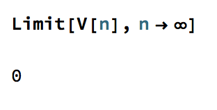
In the limit, the volume of the n-dimensional unit hypersphere tends to zero:
Now, consider the sum of the volumes of unit hypersphere in even dimensions, i.e. for n = 0, 2, 4, 6,…. For example, the first few terms of the sum are:
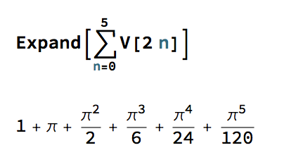
These are the initial terms of a well-known McClaurin expansion, which in the limit produces the following remarkable result:
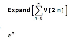
In other words, the infinite sum of the volumes of n-dimensional unit hyperspheres evaluates to a power relationship between the two most famous transcendental numbers. The result, known as Gelfond’s constant, is itself a transcendental number:
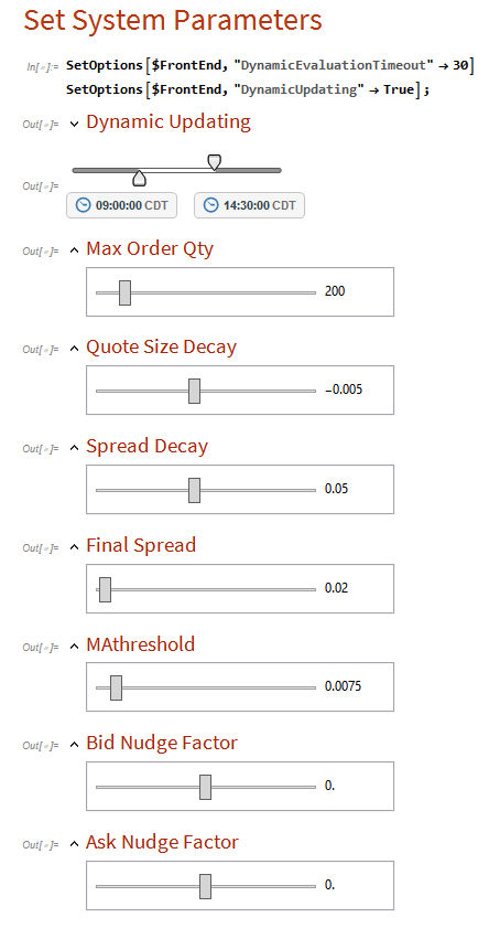
This algorithm builds on the research by Stoikova and Avelleneda in their 2009 paper “High Frequency Trading in a Limit Order Book“, 2009 and extends the basic algorithm in several ways:
The algorithm is implemented in Mathematica, and can be compiled to create dlls callable from with a C++ or Python application.
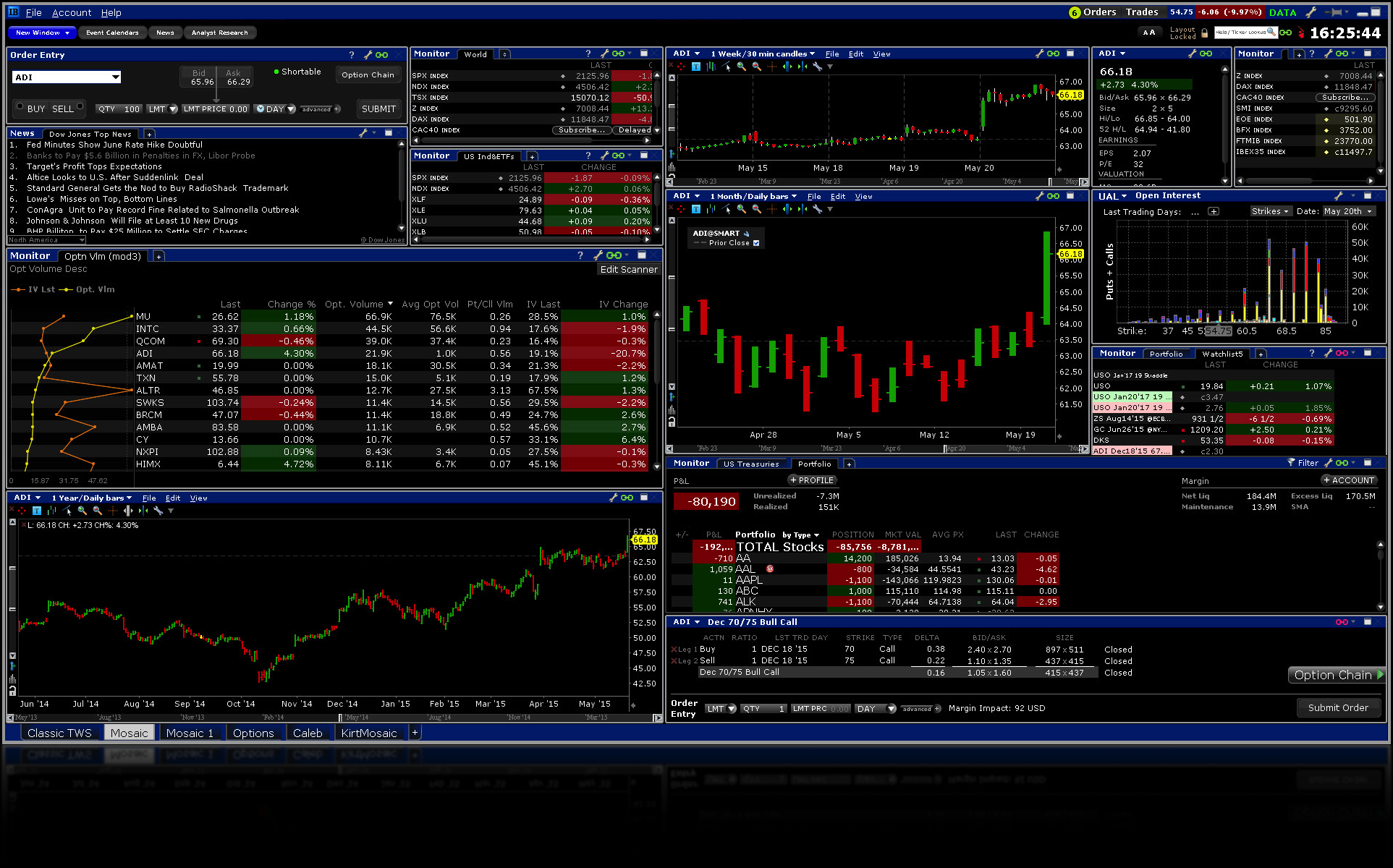
The application makes use of the MATH-TWS library to connect to the Interactive Brokers TWS or Gateway platform via the C++ api. MATH-TWS is used to create orders, manage positions and track account balances & P&L.

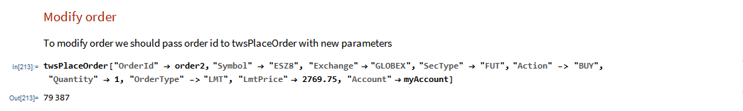
At long last, it’s here!
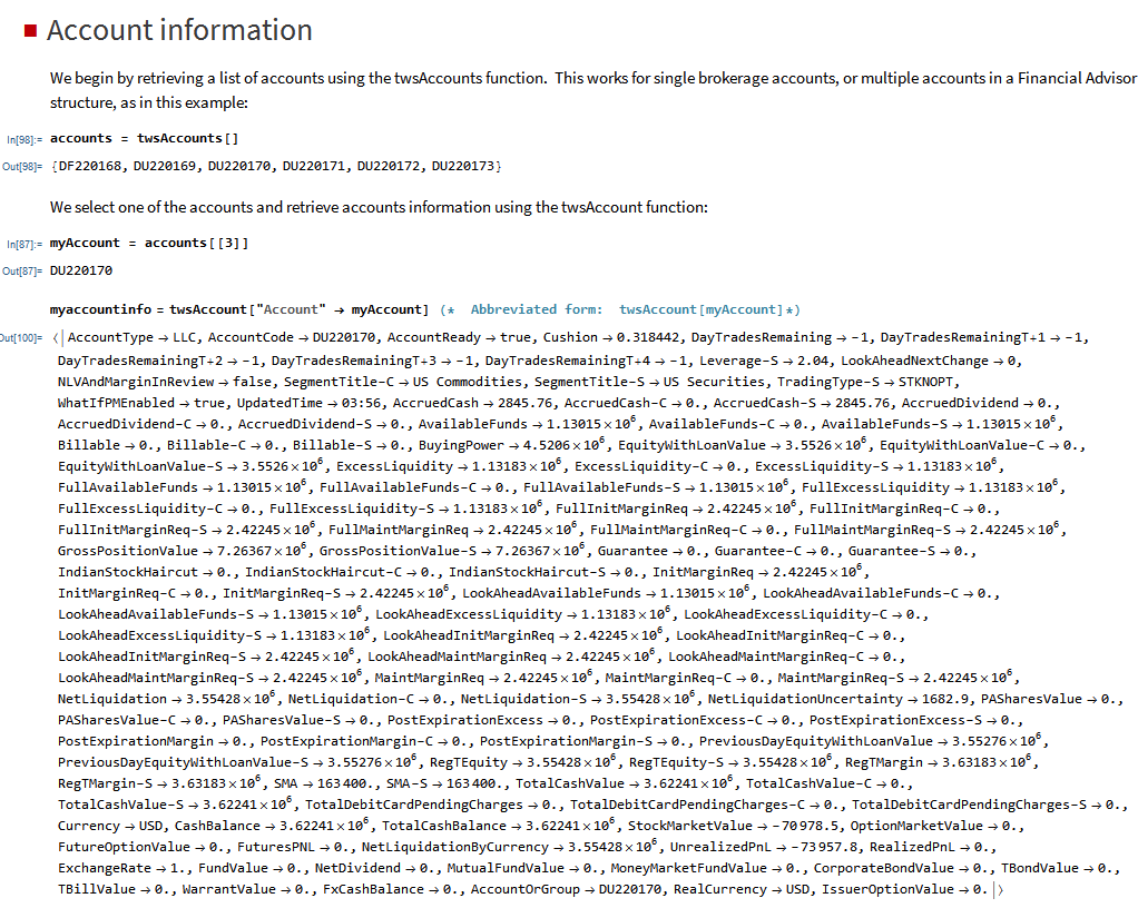
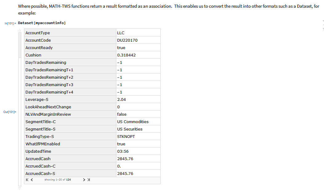
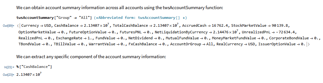
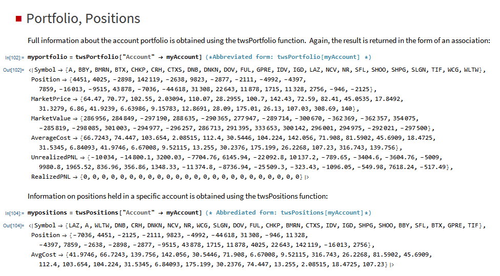
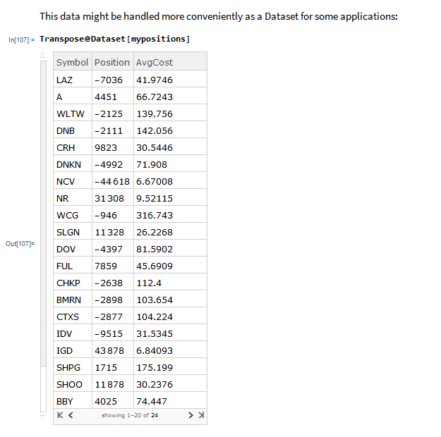
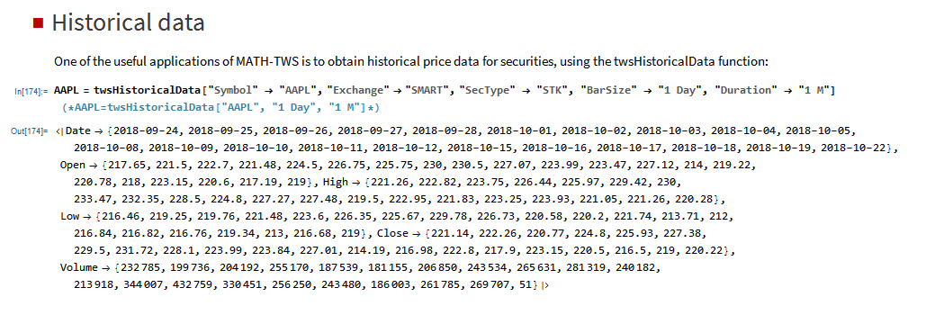
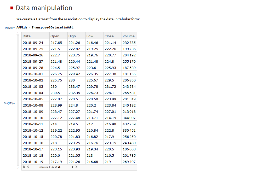
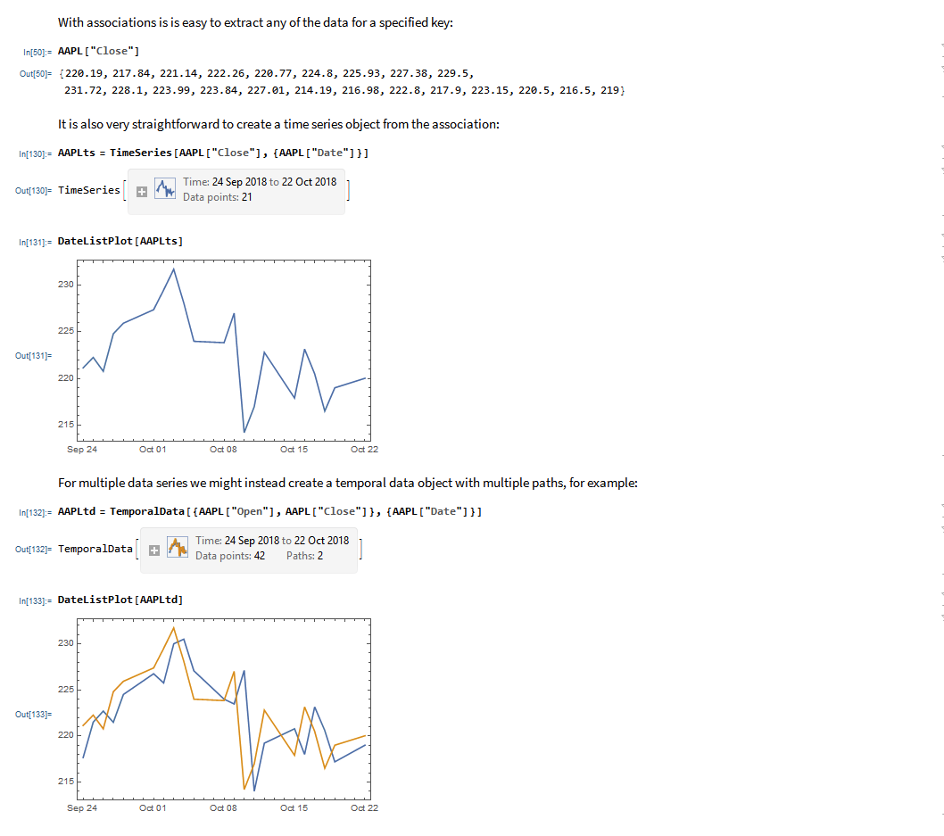
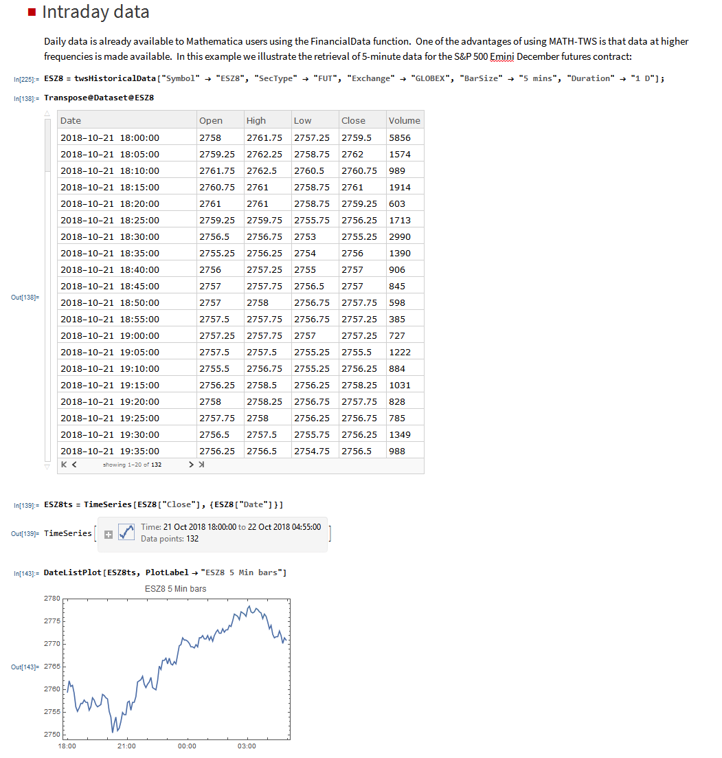
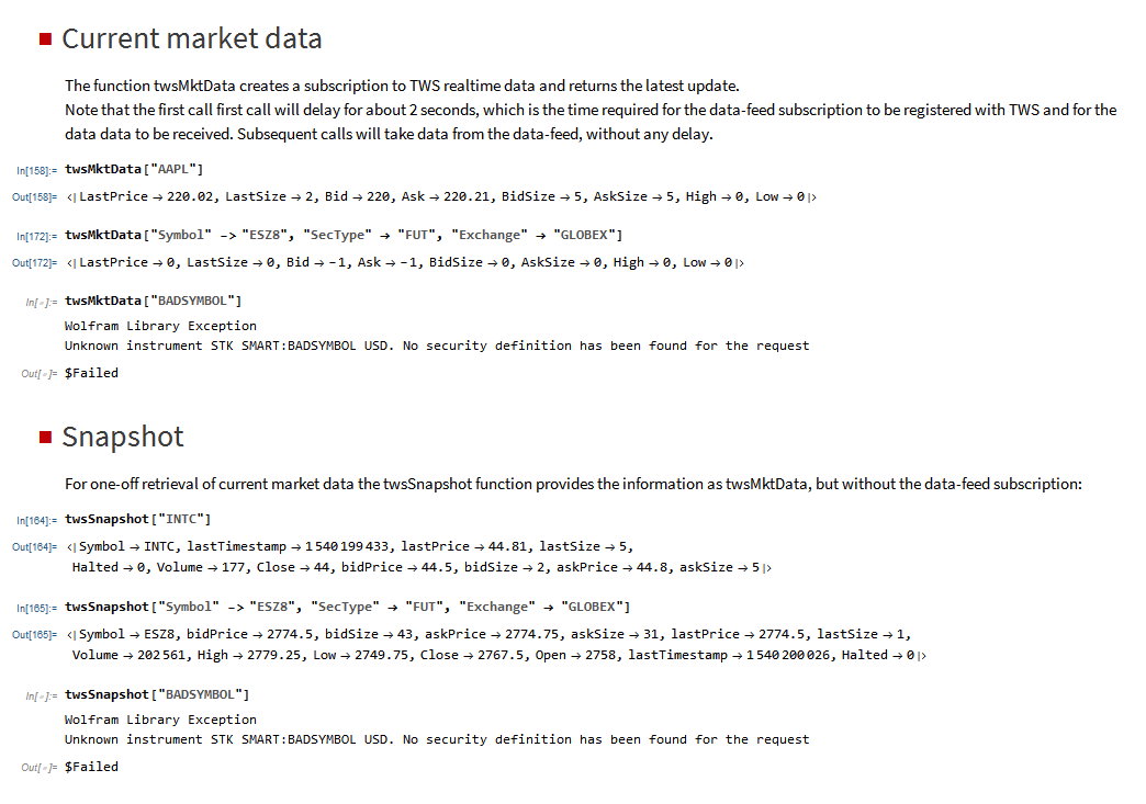
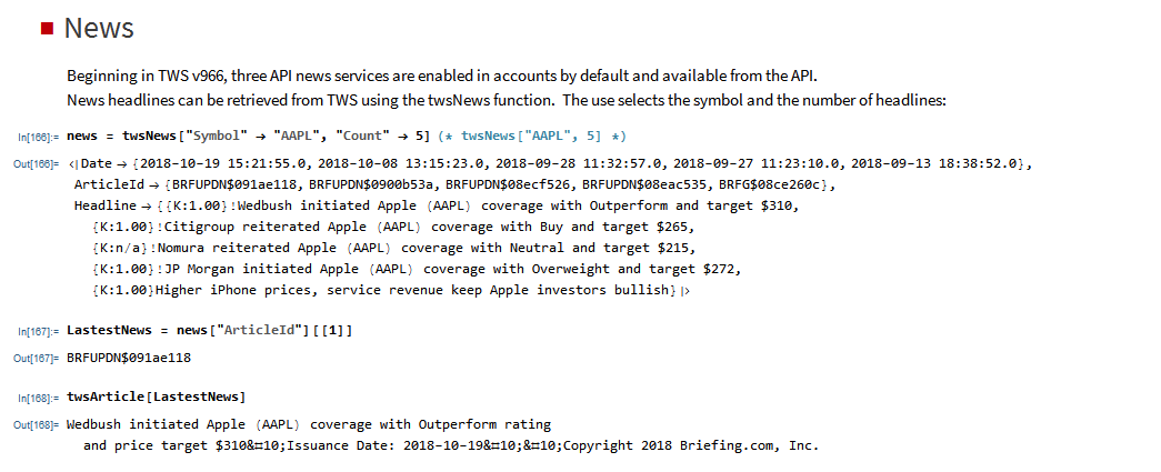
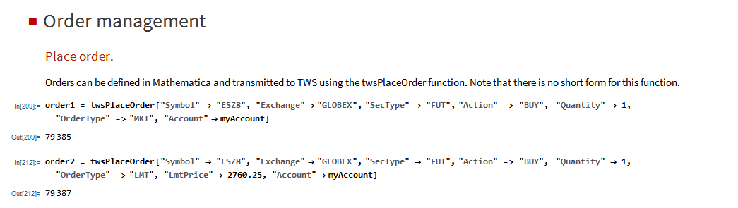
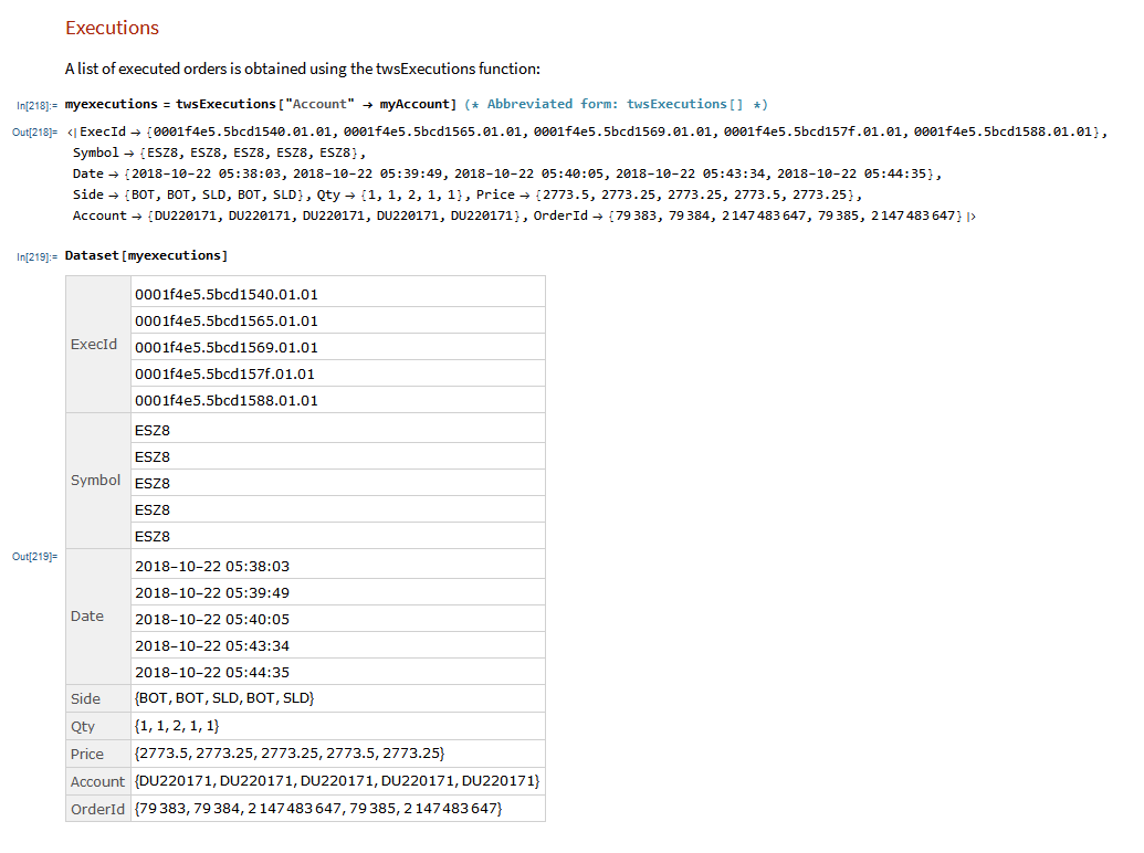
MATH-TWS is a new Mathematica package that connects Wolfram Mathematica to the Interactive Brokers TWS platform via the C++ API. It enables the user to retrieve information from TWS on accounts, portfolios and positions, as well as historical and real-time market data. MATH-TWS also enables the user to place and amend orders and obtain execution confirmations from Mathematica.
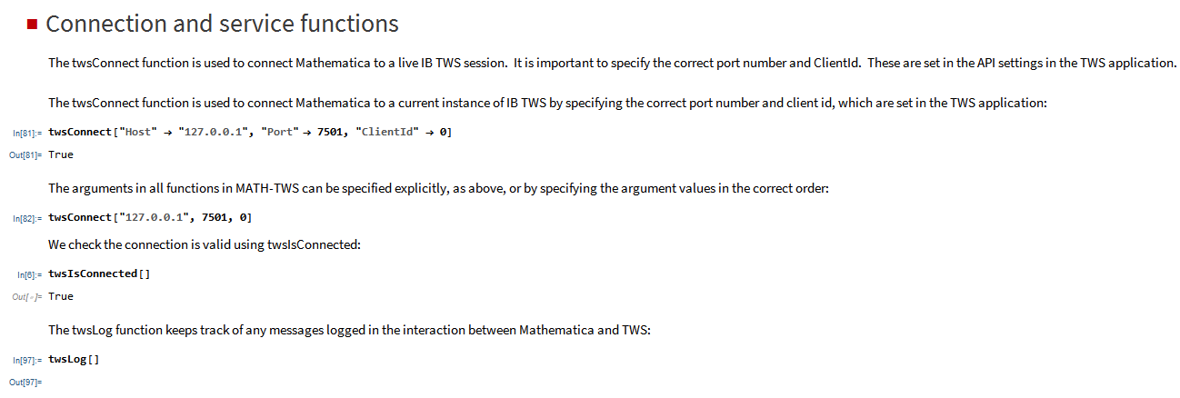
In the following sections we will illustrate the functionality of the MATH-TWS package using the full functional form and show the abbreviated equivalent form in comments.

I have wanted a way to connect Wolfram Mathematica to Interactive Brokers’ Trader Workstation for the longest time. Now that it is finally available with MATH-TWS I am excited by the possibilities for Mathematica users.
The first release of MATH-TWS will be available within a couple of weeks. Anyone interested in licensing a copy should email algorithmicexecution@gmail.com with MATH-TWS in the subject line.
Towards the end of last year I wrote a post (see here) about the advent of modern programming languages, including the JIT compiled Julia and visual programming language ADL from Trading Technologies. My conclusion (based on a not very scientific sample) was that we appear to be at the tipping point, where the speed of newer, high level languages languages is approaching that of the fastest compiled languages like C/C++.
Now comes a formal academic study of the topic in A Comparison of Programming Languages in Economics, Aruoba and Fernandez-Villaverde, 2014. Using the neoclassical growth model, the authors conduct a benchmark test in C++11, Fortran 2008, Java, Julia, Python, Matlab, Mathematica, and R, implementing the same algorithm, value function
iteration with grid search, in each of the languages. They report the execution times of the codes in a Mac and in a Windows computer and briefly comment on the strengths and weaknesses of each language.
The conclusions from the study mirror my own thoughts on the subject very closely. The authors find that:
C++ still represents the benchmark for speed, but not by much. It is barely faster than the old stalwart, Fortran, and only 1.5 – 3 times faster than up-and-coming rivals amongst the higher level languages (especially when you allow for hybrid programming to speed up the slowest algorithms).
So, as regards developing financial models and trading systems, my questions are (as before):
When you reach a point where a high level language like Matlab is only around 1.5x – 2x slower than C++, you really have to question whether the latter is an appropriate choice. Yes, of course, in mission-critical applications where you need access to the hardware layer for speed purposes, C++ is the way to go. But for so many applications, that just isn’t the case.
What matters, far, far more, are the months of costly and laborious programming effort that is often required to reproduce basic functionality that is already embedded in higher level languages like Matlab or Mathematica. Not only that, but the end result of a C++ /Java development effort is likely to be notoriously inflexible by comparison. That’s a huge drawback. Rarely, if ever, does a piece of research translate flawlessly into production – it requires one to iterate towards a final solution, often making significant changes to the design of the system in the light of practical experience.
If I had to guess, based on my experience, I would say that 80% or more of development tasks in quantitative research and trading would produce a superior result if preference was given to using a higher level language for the initial development. When the system is sufficiently stable to put into production, you simply create a hybrid application by recoding any mission-critical components for which speed is an issue in C++.
Finally, where does that leave my beloved Mathematica? To be fair, while you don’t have the joys of strong typing to contend with, Mathematica’s syntax is just as demanding and uncompromising as C++ – a missed comma or incorrectly placed bracket is just as critical. But, the point is, while in C++ the syntactical rigor is just annoying, in Mathematica it’s worth putting up with because the productivity is so much greater. A competent programmer can produce, in a single line of Mathematica code, a program that would require hundreds, if not thousands of lines of C++ code to accomplish. Sure, he might get the syntax wrong at first: but it’s only a single line of code and the interactive gui interface makes debugging very simple.
That said, while Mathematica can be very tedious to use for procedural programming, it excels in three areas:
1. Symbolic programming. Anything involving mathematical symbols and equations – Mathematica is #1
2. User interface. In Mathematica, it is trivial to build a sophisticated, dynamic gui in no time at all, again, often in 1-2 lines of code
3. Functional programming. Anything that can be thought of as a function, Mathematica handles extremely well. We are not talking about finding a square root here: I mean extremely complex functions that, again, might take hundreds of lines of code in another language.
It is also worth pointing out that Mathematica comes supplied with functionality that Matlab provides only through numerous, costly add-on packages.
CONCLUSION
Before I allow a development team to start mindlessly coding up a system in Java or C++, I want to hear their reasons why they aren’t going to do it 10x faster in another, higher level language. “We always use C++/Java for production” is not a reason. Specifically, which parts of the system require the additional 1.5x speed-up, and why can’t they be coded as dlls (Matlab mex functions)?
Finally, on a cost-benefit basis, ask yourself how much you might benefit if the months and tens (or hundreds) of thousands of dollars wasted on developing in C++ were instead spent on researching and developing new trading ideas.

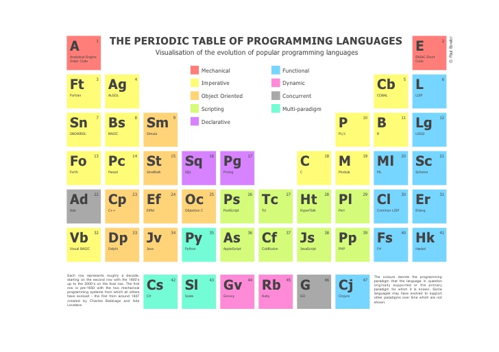
Like many in the field of quantitative research, I have programmed in several different languages over the years: Assembler, Fortran, Algol, Pascal, APL, VB, C, C++, C#, Matlab, R, Mathematica. There is an even longer list of languages I have never bothered with: Cobol, Java, Python, to name but three.
In general, the differences between many of these are much fewer than their similarities: they reserve memory; they have operators; they loop. Several have ghastly syntax requiring random punctuation that supposedly makes the code more intelligible, but in practice does precisely the opposite. Some, like Objective C, are so ugly and poorly designed they should have been strangled at birth. The ubiquity of C is due, not to its elegance, but to the fact that it was one of the first languages distributed for free to impecunious students. The greatest benefit of most languages is that they compile to machine code that executes quickly. But the task of coding in them is often an unpleasant, inefficient process that typically involves reinvention of the wheel multiple times over and massive amounts of tedious debugging. Who, after all, doesn’t enjoy unintelligible error messages like “parsec error in dynamic memory heap allocator” – when the alternative, comprehensible version would be so prosaic: “in line 51 you missed one of those curly brackets we insist on for no good reason”.
There have been relatively few steps forward that actually have had any real significance. Most times, the software industry operates rather like the motor industry: while the consumer pines for, say, a new kind of motor that will do 1,000 miles to the gallon without looking like an electric golf cart, manufacturers announce, to enormous fanfare, trivia like heated wing mirrors.

The first language I came across that seemed like a material advance was APL, a matrix-based language that offers lots of built-in functionality, very much like MatLab. Achieving useful end-results in a matter of days or weeks, rather than months, remains one of the great benefits of such high-level languages. Unfortunately, like all high-level languages that are weakly typed, APL, MatLab, R, etc, are interpreted rather than compiled. And so I learned about the perennial trade-off that has plagued systems development over the last 30 years: programming productivity vs. execution efficiency. The great divide between high level, interpreted languages and lower-level, compiled languages, would remain forever, programming language experts assured us, because of the lack of type-specificity in the former.
High-level language designers did what they could, offering ever-larger collections of sophisticated, built-in operators and libraries that use efficient machine-code instructions, as well as features such as parallel processing, to speed up execution. But, while it is now feasible to develop smaller applications in a few lines of Matlab or Mathematica that have perfectly acceptable performance characteristics, major applications (trading platforms, for example) seemed ordained to languish forever in the province of languages whose chief characteristic appears to be the lack of intelligibility of their syntax.
I was always suspicious of this thesis. It seemed to me that it should not be beyond the wit of man to design a programming language that offers straightforward, type-agnostic syntax that can be compiled. And lo: this now appears to have come true.
Of the multitude of examples that will no doubt be offered up over the next several years I want to mention two – not because I believe them to be the “final word” on this important topic, but simply as exemplars of what is now possible, as well as harbingers of what is to come.
The first, Trading Technologies’ ADL, I have written about at length already. In essence, ADL is a visual programming language focused on trading system development. ADL allows the programmer to deploy highly-efficient, pre-built code blocks as icons that are dragged and dropped onto a programming canvass and assembled together using logic connections represented by lines drawn on the canvass. From my experience, ADL outpaces any other high-level development tool by at least an order of magnitude, but without sacrificing (much) efficiency in execution, firstly because the code blocks are written in native C#, and secondly, because completed systems are deployed on an algo server with a sub-millisecond connectivity to the exchange.

The second example is a language called Julia, which you can find out more about here. To quote from the web site:
“Julia is a high-level, high-performance dynamic programming language for technical computing. Julia features optional typing, multiple dispatch, and good performance, achieved using type inference and just-in-time (JIT) compilation, implemented using LLVM”
The language syntax is indeed very straightforward and logical. As to performance, the evidence appears to be that it is possible to achieve execution speeds that match or even exceed those achieved by languages like Java or C++.
The following micro-benchmark results, provided on the Julia web site, were obtained on a single core (serial execution) on an Intel® Xeon® CPU E7-8850 2.00GHz CPU with 1TB of 1067MHz DDR3 RAM, running Linux:
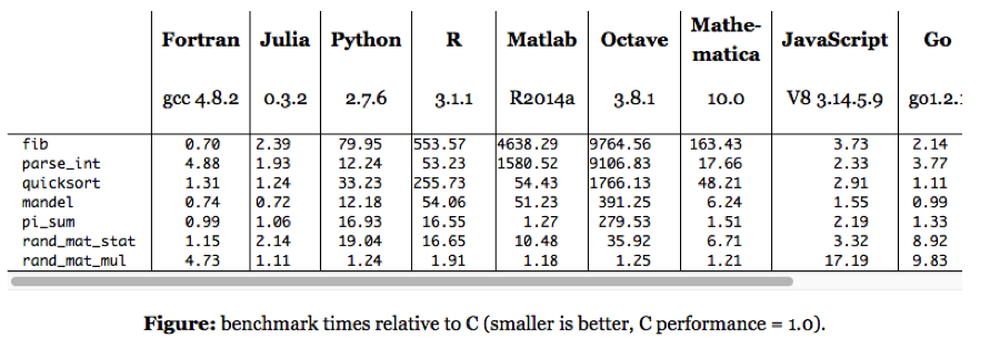
We need not pretend that this represents any kind of comprehensive speed test of Julia or its competitors. Still, it’s worth dwelling on a few of the salient results. The first thing that strikes me is how efficient Fortran, the grand-daddy of programming languages, remains in comparison to more modern alternatives, including the C benchmark. The second result I find striking is how slow the much-touted Python is compared to Julia, Go and C. The third result is how poorly MatLab, Octave and R perform on several of the tests. Finally, and in some ways the greatest surprise at all is the execution efficiency of Mathematica relative to other high-level languages like MatLab and R. It appears that Wolfram has made enormous progress in improving the speed of Mathematica, presumably through the vast expansion of highly efficient built-in operators and functions that have been added in recent releases (see chart below).
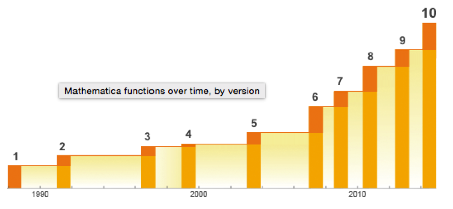
Source: Wolfram
Mathematica even compares favorably to Python on several of the tests. Given that, why would anyone spend time learning a language like Python, which offers neither the development advantages of Mathematica, nor the speed advantages of C (or Fortran, Java or Julia)?
In any event, the main point is this: it appears that, in 2015, we can finally look forward to dispensing with legacy programing languages and their primitive syntax and instead develop large, scalable systems that combine programming productivity and execution efficiency. And that is reason enough for any self-respecting quant to rejoice.
My best wishes to you all for the New Year.
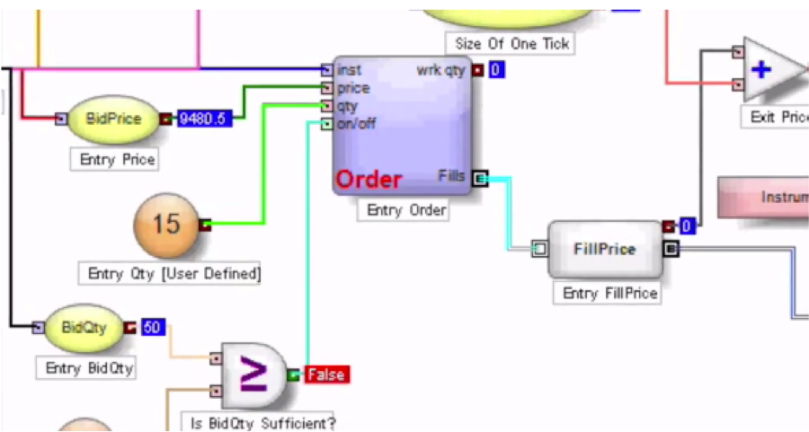
Trading Technologies’ ADL is a visual programming language designed specifically for trading strategy development that is integrated in the company’s flagship XTrader product. 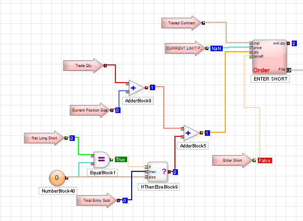 Despite the radically different programming philosophy, my experience of working with ADL has been delightfully easy and strategies that would typically take many months of coding in C++ have been up and running in a matter of days or weeks. An extract of one such strategy, a high frequency scalping trade in the E-Mini S&P 500 futures, is shown in the graphic above. The interface and visual language is so intuitive to a trading system developer that even someone who has never seen ADL before can quickly grasp at least some of what it happening in the code.
Strategy Development in Low vs. High-Level Languages
What are the benefits of using a high level language like ADL compared to programming languages like C++/C# or Java that are traditionally used for trading system development? The chief advantage is speed of development: I would say that ADL offers the potential up the development process by at least one order of magnitude. A complex trading system would otherwise take months or even years to code and test in C++ or Java, can be implemented successfully and put into production in a matter of weeks in ADL. In this regard, the advantage of speed of development is one shared by many high level languages, including, for example, Matlab, R and Mathematica. But in ADL’s case the advantage in terms of time to implementation is aided by the fact that, unlike generalist tools such as MatLab, etc, ADL is designed specifically for trading system development. The ADL development environment comes equipped with compiled pre-built blocks designed to accomplish many of the common tasks associated with any trading system such as acquiring market data and handling orders. Even complex spread trades can be developed extremely quickly due to the very comprehensive library of pre-built blocks.
Integrating Research and Development
One of the drawbacks of using a higher level language for building trading systems is that, being interpreted rather than compiled, they are simply too slow – one or more orders of magnitude, typically – to be suitable for high frequency trading. I will come on to discuss the execution speed issue a little later. For now, let me bring up a second major advantage of ADL relative to other high level languages, as I see it. One of the issues that plagues trading system development is the difficulty of communication between researchers, who understand financial markets well, but systems architecture and design rather less so, and developers, whose skill set lies in design and programming, but whose knowledge of markets can often be sketchy. These difficulties are heightened where researchers might be using a high level language and relying on developers to re-code their prototype system to get it into production. Developers typically (and understandably) demand a high degree of specificity about the requirement and if it’s not included in the spec it won’t be in the final deliverable. Unfortunately, developing a successful trading system is a highly non-linear process and a researcher will typically have to iterate around the core idea repeatedly until they find a combination of alpha signal and entry/exit logic that works. In other words, researchers need flexibility, whereas developers require specificity. ADL helps address this issue by providing a development environment that is at once highly flexible and at the same time powerful enough to meet the demands of high frequency trading in a production environment. It means that, in theory, researchers and developers can speak a common language and use a common tool throughout the R&D development cycle. This is likely to reduce the kind of misunderstanding between researchers and developers that commonly arise (often setting back the implementation schedule significantly when they do).
Latency
Of course, at least some of the theoretical benefit of using ADL depends on execution speed. The way the problem is typically addressed with systems developed in high level languages like Matlab or R is to recode the entire system in something like C++, or to recode some of the most critical elements and plug those back into the main Matlab program as dlls. The latter approach works, and preserves the most important benefits of working in both high and low level languages, but the resulting system is likely to be sub-optimal and can be difficult to maintain. The approach taken by Trading Technologies with ADL is very different. Firstly, the component blocks are written in C# and in compiled form should run about as fast as native code. Secondly, systems written in ADL can be deployed immediately on a co-located algo server that is plugged directly into the exchange, thereby reducing latency to an acceptable level. While this is unlikely to sufficient for an ultra-high frequency system operating on the sub-millisecond level, it will probably suffice for high frequency systems that operate at speeds above above a few millisecs, trading up to say, around 100 times a day.
Fill Rate and Toxic Flow
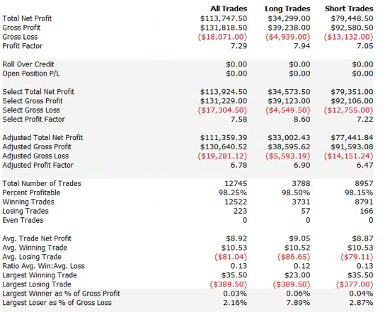
For those not familiar with the HFT territory, let me provide an example of why the issues of execution speed and latency are so important. Below is a simulated performance record for a HFT system in ES futures. The system is designed to enter and exit using limit orders and trades around 120 times a day, with over 98% profitability, if we assume a 100% fill rate. 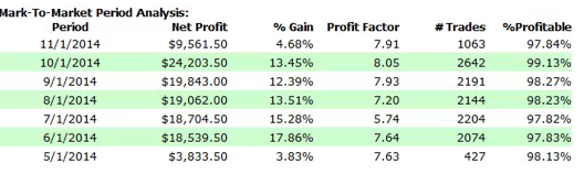
 So far so good. But a 100% fill rate is clearly unrealistic. Let’s look at a pessimistic scenario: what if we got filled on orders only when the limit price was exceeded? (For those familiar with the jargon, we are assuming a high level of flow toxicity) The outcome is rather different:
 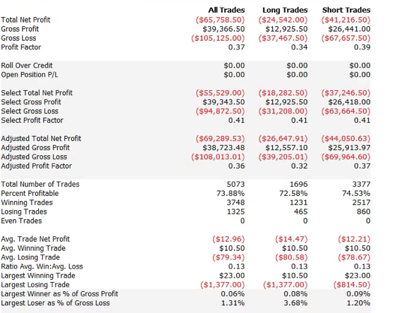 Neither scenario is particularly realistic, but the outcome is much more likely to be closer to the second scenario rather than the first if we our execution speed is slow, or if we are using a retail platform such as Interactive Brokers or Tradestation, with long latency wait times. The reason is simple: our orders will always arrive late and join the limit order book at the back of the queue. In most cases the orders ahead of ours will exhaust demand at the specified limit price and the market will trade away without filling our order. At other times the market will fill our order whenever there is a large flow against us (i.e. a surge of sell orders into our limit buy), i.e. when there is significant toxic flow. The proposition is that, using ADL and the its high-speed trading infrastructure, we can hope to avoid the latter outcome. While we will never come close to achieving a 100% fill rate, we may come close enough to offset the inevitable losses from toxic flow and produce a decent return. Whether ADL is capable of fulfilling that potential remains to be seen.
More on ADL
For more information on ADL go here.

In this quantitative analysis I explore how, starting from the assumption of a stable, Gaussian distribution in a returns process, we evolve to a system that displays all the characteristics of empirical market data, notably time-dependent moments, high levels of kurtosis and fat tails. As it turns out, the only additional assumption one needs to make is that the market is periodically disturbed by the random arrival of news.
NOTE: if you are unable to see the Mathematica models below, you can download the free Wolfram CDF player and you may also need this plug-in.
You can also download the complete Mathematica CDF file here.
A stationary process is one that evolves over time, but whose probability distribution does not vary with time. As the word implies, such a process is stable. More formally, the moments of the distribution are independent of time.
Let’s assume we are dealing with such a process that have constant mean μ and constant volatility (standard deviation) σ.
Φ=NormalDistribution[μ,σ]
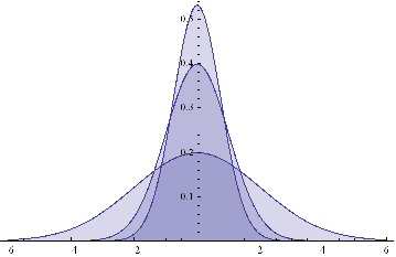
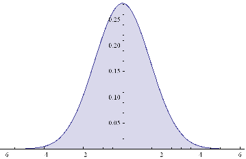
Here are some examples of Normal probability distributions, with constant mean μ = 0 and standard deviation σ ranging from 0.75 to 2
Plot[Evaluate@Table[PDF[Φ,x],{σ,{.75,1,2}}]/.μ→0,{x,-6,6},Filling→Axis]
The moments of Φ are given by:
Through[{Mean, StandardDeviation, Skewness, Kurtosis}[Φ]]
{μ, σ, 0, 3}
They, too, are time – independent.
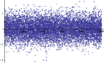
We can simulate some observations from such a process, with, say, mean μ = 0 and standard deviation σ = 1:
ListPlot[sampleData=RandomVariate[Φ /.{μ→0, σ→1},10^4]]
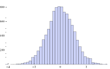
Histogram[sampleData]
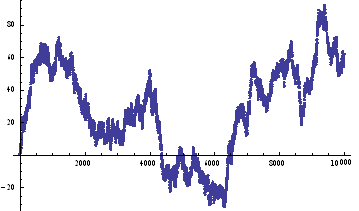
If we assume for the moment that such a process is an adequate description of an asset returns process, we can simulate the evolution of a price process as follows :
ListPlot[prices=Accumulate[sampleData]]
Lets take a look at a real price series, comprising 1 – minute bar data in the June ‘ 14 E – Mini futures contract.
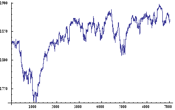
As with our simulated price process, it is clear that the real price process for Emini futures is also non – stationary.
What about the returns process?
ListPlot[returnsES]
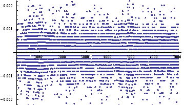
Notice the banding effect in returns, which results from having a fixed, minimum price move of $12 .50, rather than a continuous scale.
Histogram[returnsES]
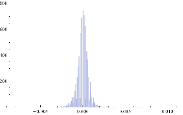
Through[{Min,Max,Mean,Median,StandardDeviation,Skewness,Kurtosis}[returnsES]]
{-0.00867214, 0.0112353, 2.75501×10⁻⁶, 0., 0.000780895, 0.35467, 26.2376}
The empirical returns distribution doesn’ t appear to be Gaussian – the distribution is much more peaked than a standard Normal distribution with the same mean and standard deviation. And the higher moments don’t fit the Normal model either – the empirical distribution has positive skew and a kurtosis that is almost 9x greater than a Gaussian distribution. The latter signifies what is often referred to as “fat tails”: the distribution has much greater weight in the tails than a standard Normal distribution, indicating a much greater likelihood of an extreme value than a Normal distribution would predict.
Non – stationarity arises when one or more of the moments of a distribution vary over time. Let’s take a look at how that can arise, and its effects.Suppose we have a Gaussian returns process for which the mean, or drift, or trend, fluctuates over time.
Let’s consider a simple example where the process drift is μ1 and volatility σ1 for most of the time and then for some proportion of time k, we get addition drift μ2 and volatility σ2. In other words we have:
Φ1=NormalDistribution[μ1,σ1]
Through[{Mean,StandardDeviation,Skewness,Kurtosis}[Φ1]]
{μ1, σ1, 0, 3}
Φ2=NormalDistribution[μ2,σ2]
Through[{Mean,StandardDeviation,Skewness,Kurtosis}[Φ2]]
{μ2, σ2, 0, 3}
This simple model fits a scenario in which we suppose that the returns process spends most of its time in State 1, in which is Normally distributed with drift is μ1 and volatility σ1, and suffers from the occasional “shock” which propels the systems into a second State 2, in which its distribution is a combination of its original distribution and a new Gaussian distribution with different mean and volatility.
Let’ s suppose that we sample the combined process y = Φ1 + k Φ2. What distribution would it have? We can represent this is follows :
y=TransformedDistribution[(x1+k x2),{x1~Φ1,x2~Φ2}]
Through[{Mean,StandardDeviation,Skewness,Kurtosis}[y]]
![]()
Plot[PDF[y,x]/.{μ1→0,μ2→0,σ1 →1,σ2 →2, k→0.5},{x,-6,6},Filling→Axis]
The result is just another Normal distribution. Depending on the incidence k, y will follow a Gaussian distribution whose mean and variance depend on the mean and variance of the two Normal distributions being mixed. The resulting distribution in State 2 may have higher or lower drift and volatility, but it is still Gaussian, with constant kurtosis of 3.
In other words, the system y will be non-stationary, because the first and second moments change over time, depending on what state it is in. But the form of the distribution is unchanged – it is still Gaussian. There are no fat-tails.
In the above example the system moved between states in a known, predictable way. The “shocks” to the system were not really shocks, but transitions. But that’s not how financial markets behave: markets move from one state to another in an unpredictable way, with the arrival of news.
We can simulate this situation as follows. Using the former model as a starting point, lets now relax the assumption that the incidence of the second state, k, is a constant. Instead, let’ s assume that k is itself a random variable. In other words we are going to now assume that our system changes state in a random way. How does this alter the distribution?
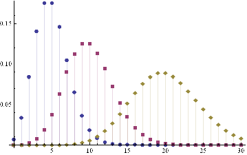
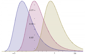
An appropriate model for λ might be a Poisson process, which is often used as a model for unpredictable, discrete events, ranging from bus arrivals to earthquakes. PDFs of Poisson distributions with means λ=5, 10 and 20 are shown in the chart below. These represent probability distributions for processes that have mean arrivals of 5, 10 or 20 events.
DiscretePlot[Evaluate@Table[PDF[PoissonDistribution[λ],k],{λ,{5,10,20}}],{k,0,30},PlotRange→All,PlotMarkers→Automatic]
Our new model now looks like this :
y=TransformedDistribution[{x1+k*x2},{x1⎡Φ1,x2⎡Φ2,k⎡PoissonDistribution[λ]}]
The first two moments of the distribution are as follows :
Through[{Mean,StandardDeviation}[y]]
![]()
As before, the mean and standard deviation of the distribution are going to vary, depending on the state of the system, and the mean arrival rate of shocks, . But what about kurtosis? Is it still constant?
Kurtosis[y]
Emphatically not! The fourth moment of the distribution is now dependent on the drift in the second state, the volatilities of both states and the mean arrival rate of shocks, λ.
Let’ s look at a specific example. Assume that in State 1 the process has volatility of 7.5 %, with zero drift, and that the shock distribution also has zero drift with volatility of 65 %. If the mean incidence rate of shocks λ = 10 %, the distribution kurtosis is close to that seen in the empirical distribution for the E-Mini.
Kurtosis[y] /.{σ1→0.075,μ2→0,σ2→0.65,λ→0.1}
{35.3551}
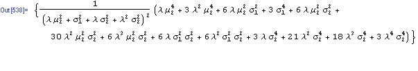
More generally :
ListLinePlot[Flatten[Kurtosis[y]/.Table[{σ1→0.075,μ2→0,σ2→0.65,λ→i/20},{i,1,20}]],PlotLabel→Style[“Kurtosis vs Mean Shock Arrival Rate”, FontSize→18],AxesLabel->{“Incidence Rate (%)”, “Kurtosis”},Filling→Axis, ImageSize→Large]
Thus we can see how, even if the underlying returns distribution is Gaussian in form, the random arrival of news “shocks” to the system can induce non – stationarity in overall drift and volatility. It can also result in fat tails. More specifically, if the arrival of news is stochastic in nature, rather than deterministic, the process may exhibit far higher levels of kurtosis than in its original Gaussian state, in which the fourth moment was a constant level of 3.
Nobel – prize winning economist Robert Merton extended this basic concept to the realm of stochastic calculus.
In Merton’s jump diffusion model, the stock price follows the random process
∂St / St =μdt + σdWt+(J-1)dNt
The first two terms are familiar from the Black–Scholes model : drift rate μ, volatility σ, and random walk Wt (Wiener process).The last term represents the jumps :J is the jump size as a multiple of stock price, while Nt is the number of jump events that have occurred up to time t.is assumed to follow the Poisson process.
PDF[PoissonDistribution[λt]]
where λ is the average frequency with which jumps occur.
The jump size J follows a log – normal distribution
PDF[LogNormalDistribution[m, ν], s]
where m is the average jump size and v is the volatility of the jump size.
In the jump diffusion model, the stock price St follows the random process dSt/St=μ dt+σ dWt+(J-1) dN(t), which comprises, in order, drift, diffusive, and jump components. The jumps occur according to a Poisson distribution and their size follows a log-normal distribution. The model is characterized by the diffusive volatility σ, the average jump size J (expressed as a fraction of St), the frequency of jumps λ, and the volatility of jump size ν.
The “implied volatility” corresponding to an option price is the value of the volatility parameter for which the Black-Scholes model gives the same price. A well-known phenomenon in market option prices is the “volatility smile”, in which the implied volatility increases for strike values away from the spot price. The jump diffusion model is a generalization of Black–Scholes in which the stock price has randomly occurring jumps in addition to the random walk behavior. One of the interesting properties of this model is that it displays the volatility smile effect. In this Demonstration, we explore the Black–Scholes implied volatility of option prices (equal for both put and call options) in the jump diffusion model. The implied volatility is modeled as a function of the ratio of option strike price to spot price.
NOTE: if you are unable to see the Mathematica models below, you can download the free Wolfram CDF player and you may also need this plug-in.
You can also download the complete Mathematica CDF file here.
In this post I want to explore aspects of scalping, a type of strategy widely utilized by high frequency trading firms.
I will define a scalping strategy as one in which we seek to take small profits by posting limit orders on alternate side of the book. Scalping, as I define it, is a strategy rather like market making, except that we “lean” on one side of the book. So, at any given time, we may have a long bias and so look to enter with a limit buy order. If this is filled, we will then look to exit with a subsequent limit sell order, taking a profit of a few ticks. Conversely, we may enter with a limit sell order and look to exit with a limit buy order.
The strategy relies on two critical factors:
(i) the alpha signal which tells us from moment to moment whether we should prefer to be long or short
(ii) the execution strategy, or “trade expression”
In this article I want to focus on the latter, making the assumption that we have some kind of alpha generation model already in place (more about this in later posts).
There are several means that a trader can use to enter a position. The simplest approach, the one we will be considering here, is simply to place a single limit order at or just outside the inside bid/ask prices – so in other words we will be looking to buy on the bid and sell on the ask (and hoping to earn the bid-ask spread, at least).
One of the problems with this approach is that it is highly latency sensitive. Limit orders join the limit order book at the back of the queue and slowly works their way towards the front, as earlier orders get filled. Buy the time the market gets around to your limit buy order, there may be no more sellers at that price. In that case the market trades away, a higher bid comes in and supersedes your order, and you don’t get filled. Conversely, yours may be one of the last orders to get filled, after which the market trades down to a lower bid and your position is immediately under water.
This simplistic model explains why latency is such a concern – you want to get as near to the front of the queue as you can, as quickly as possible. You do this by minimizing the time it takes to issue and order and get it into the limit order book. That entails both hardware (co-located servers, fiber-optic connections) and software optimization and typically also involves the use of Immediate or Cancel (IOC) orders. The use of IOC orders by HFT firms to gain order priority is highly controversial and is seen as gaming the system by traditional investors, who may end up paying higher prices as a result.
Another approach is to layer limit orders at price points up and down the order book, establishing priority long before the market trades there. Order layering is a highly complex execution strategy that brings addition complications.
Let’s confine ourselves to considering the single limit order, the type of order available to any trader using a standard retail platform.
As I have explained, we are assuming here that, at any point in time, you know whether you prefer to be long or short, and therefore whether you want to place a bid or an offer. The issue is, at what price do you place your order, and what do you do about limiting your risk? In other words, we are discussing profit targets and stop losses, which, of course, are all about risk and return.
Lets start by considering risk. The biggest risk to a scalper is that, once filled, the market goes against his position until he is obliged to trigger his stop loss. If he sets his stop loss too tight, he may be forced to exit positions that are initially unprofitable, but which would have recovered and shown a profit if he had not exited. Conversely, if he sets the stop loss too loose, the risk reward ratio is very low – a single loss-making trade could eradicate the profit from a large number of smaller, profitable trades.
Now lets think about reward. If the trader is too ambitious in setting his profit target he may never get to realize the gains his position is showing – the market could reverse, leaving him with a loss on a position that was, initially, profitable. Conversely, if he sets the target too tight, the trader may give up too much potential in a winning trade to overcome the effects of the occasional, large loss.
It’s clear that these are critical concerns for a scalper: indeed the trade exit rules are just as important, or even more important, than the entry rules. So how should he proceed?
Let’s make the rather heroic assumption that market returns are Normally distributed (in fact, we know from empirical research that they are not – but this is a starting point, at least). And let’s assume for the moment that our trader has been filled on a limit buy order and is looking to decide where to place his profit target and stop loss limit orders. Given a current price of the underlying security of X, the scalper is seeking to determine the profit target of p ticks and the stop loss level of q ticks that will determine the prices at which he should post his limit orders to exit the trade. We can translate these into returns, as follows:
to the upside: Ru = Ln[X+p] – Ln[X]
and to the downside: Rd = Ln[X-q] – Ln[X]
This situation is illustrated in the chart below.
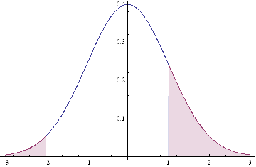
The profitable area is the shaded region on the RHS of the distribution. If the market trades at this price or higher, we will make money: p ticks, less trading fees and commissions, to be precise. Conversely we lose q ticks (plus commissions) if the market trades in the region shaded on the LHS of the distribution.
Under our assumptions, the probability of ending up in the RHS shaded region is:
probWin = 1 – NormalCDF(Ru, mu, sigma),
where mu and sigma are the mean and standard deviation of the distribution.
The probability of losing money, i.e. the shaded area in the LHS of the distribution, is given by:
probLoss = NormalCDF(Rd, mu, sigma),
where NormalCDF is the cumulative distribution function of the Gaussian distribution.
The expected profit from the trade is therefore:
Expected profit = p * probWin – q * probLoss
And the expected win rate, the proportion of profitable trades, is given by:
WinRate = probWin / (probWin + probLoss)
If we set a stretch profit target, then p will be large, and probWin, the shaded region on the RHS of the distribution, will be small, so our winRate will be low. Under this scenario we would have a low probability of a large gain. Conversely, if we set p to, say, 1 tick, and our stop loss q to, say, 20 ticks, the shaded region on the RHS will represent close to half of the probability density, while the shaded LHS will encompass only around 5%. Our win rate in that case would be of the order of 91%:
WinRate = 50% / (50% + 5%) = 91%
Under this scenario, we make frequent, small profits and suffer the occasional large loss.
So the critical question is: how do we pick p and q, our profit target and stop loss? Does it matter? What should the decision depend on?
We can begin to address these questions by noticing, as we have already seen, that there is a trade-off between the size of profit we are hoping to make, and the size of loss we are willing to tolerate, and the probability of that gain or loss arising. Those probabilities in turn depend on the underlying probability distribution, assumed here to be Gaussian.
Now, the Normal or Gaussian distribution which determines the probabilities of winning or losing at different price levels has two parameters – the mean, mu, or drift of the returns process and sigma, its volatility.
Over short time intervals the effect of volatility outweigh any impact from drift by orders of magnitude. The reason for this is simple: volatility scales with the square root of time, while the drift scales linearly. Over small time intervals, the drift becomes un-noticeably small, compared to the process volatility. Hence we can assume that mu, the process mean is zero, without concern, and focus exclusively on sigma, the volatility.
What other factors do we need to consider? Well there is a minimum price move, which might be 1 tick, and the dollar value of that tick, from which we can derive our upside and downside returns, Ru and Rd. And, finally, we need to factor in commissions and exchange fees into our net trade P&L.
Here’s a simple formulation of the model, in which I am using the E-mini futures contract as an exemplar.
WinRate[currentPrice_,annualVolatility_,BarSizeMins_, nTicksPT_, nTicksSL_,minMove_, tickValue_, costContract_]:=Module[{ nMinsPerDay, periodVolatility, tgtReturn, slReturn,tgtDollar, slDollar, probWin, probLoss, winRate, expWinDollar, expLossDollar, expProfit},
nMinsPerDay = 250*6.5*60;
periodVolatility = annualVolatility / Sqrt[nMinsPerDay/BarSizeMins];
tgtReturn=nTicksPT*minMove/currentPrice;tgtDollar = nTicksPT * tickValue;
slReturn = nTicksSL*minMove/currentPrice;
slDollar=nTicksSL*tickValue;
probWin=1-CDF[NormalDistribution[0, periodVolatility],tgtReturn];
probLoss=CDF[NormalDistribution[0, periodVolatility],slReturn];
winRate=probWin/(probWin+probLoss);
expWinDollar=tgtDollar*probWin;
expLossDollar=slDollar*probLoss;
expProfit=expWinDollar+expLossDollar-costContract;
{expProfit, winRate}]
For the ES contract we have a min price move of 0.25 and the tick value is $12.50. Notice that we scale annual volatility to the size of the period we are trading (15 minute bars, in the following example).
Let’s take a look at how the expected profit and win rate vary with the profit target and stop loss limits we set. In the following interactive graphics, we can assess the impact of different levels of volatility on the outcome.
Notice to begin with that the win rate (and expected profit) are very far from being Normally distributed – not least because they change radically with volatility, which is itself time-varying.
For very low levels of volatility, around 5%, we appear to do best in terms of maximizing our expected P&L by setting a tight profit target of a couple of ticks, and a stop loss of around 10 ticks. Our win rate is very high at these levels – around 90% or more. In other words, at low levels of volatility, our aim should be to try to make a large number of small gains.
But as volatility increases to around 15%, it becomes evident that we need to increase our profit target, to around 10 or 11 ticks. The distribution of the expected P&L suggests we have a couple of different strategy options: either we can set a larger stop loss, of around 30 ticks, or we can head in the other direction, and set a very low stop loss of perhaps just 1-2 ticks. This later strategy is, in fact, the mirror image of our low-volatility strategy: at higher levels of volatility, we are aiming to make occasional, large gains and we are willing to pay the price of sustaining repeated small stop-losses. Our win rate, although still well above 50%, naturally declines.
As volatility rises still further, to 20% or 30%, or more, it becomes apparent that we really have no alternative but to aim for occasional large gains, by increasing our profit target and tightening stop loss limits. Our win rate under this strategy scenario will be much lower – around 30% or less.
Now let’s address the concern that asset returns are not typically distributed Normally. In particular, the empirical distribution of returns tends to have “fat tails”, i.e. the probability of an extreme event is much higher than in an equivalent Normal distribution.
A widely used model for fat-tailed distributions in the Extreme Value Distribution. This has pdf:
PDF[ExtremeValueDistribution[,],x]

Plot[Evaluate@Table[PDF[ExtremeValueDistribution[,2],x],{,{-3,0,4}}],{x,-8,12},FillingAxis]
Mean[ExtremeValueDistribution[,]]
+EulerGamma
Variance[ExtremeValueDistribution[,]]
![]()
In order to set the parameters of the EVD, we need to arrange them so that the mean and variance match those of the equivalent Gaussian distribution with mean = 0 and standard deviation . hence:
![]()
The code for a version of the model using the GED is given as follows
WinRateExtreme[currentPrice_,annualVolatility_,BarSizeMins_, nTicksPT_, nTicksSL_,minMove_, tickValue_, costContract_]:=Module[{ nMinsPerDay, periodVolatility, alpha, beta,tgtReturn, slReturn,tgtDollar, slDollar, probWin, probLoss, winRate, expWinDollar, expLossDollar, expProfit},
nMinsPerDay = 250*6.5*60;
periodVolatility = annualVolatility / Sqrt[nMinsPerDay/BarSizeMins];
beta = Sqrt[6]*periodVolatility / Pi;
alpha=-EulerGamma*beta;
tgtReturn=nTicksPT*minMove/currentPrice;tgtDollar = nTicksPT * tickValue;
slReturn = nTicksSL*minMove/currentPrice;
slDollar=nTicksSL*tickValue;
probWin=1-CDF[ExtremeValueDistribution[alpha, beta],tgtReturn];
probLoss=CDF[ExtremeValueDistribution[alpha, beta],slReturn];
winRate=probWin/(probWin+probLoss);
expWinDollar=tgtDollar*probWin;
expLossDollar=slDollar*probLoss;
expProfit=expWinDollar+expLossDollar-costContract;
{expProfit, winRate}]
WinRateExtreme[1900,0.05,15,2,30,0.25,12.50,3][[2]]
0.21759
We can now produce the same plots for the EVD version of the model that we plotted for the Gaussian versions :
Next we compare the Gaussian and EVD versions of the model, to gain an understanding of how the differing assumptions impact the expected Win Rate.
As you can see, for moderate levels of volatility, up to around 18 % annually, the expected Win Rate is actually higher if we assume an Extreme Value distribution of returns, rather than a Normal distribution.If we use a Normal distribution we will actually underestimate the Win Rate, if the actual return distribution is closer to Extreme Value.In other words, the assumption of a Gaussian distribution for returns is actually conservative.
Now, on the other hand, it is also the case that at higher levels of volatility the assumption of Normality will tend to over – estimate the expected Win Rate, if returns actually follow an extreme value distribution. But, as indicated before, for high levels of volatility we need to consider amending the scalping strategy very substantially. Either we need to reverse it, setting larger Profit Targets and tighter Stops, or we need to stop trading altogether, until volatility declines to normal levels.Many scalpers would prefer the second option, as the first alternative doesn’t strike them as being close enough to scalping to justify the name.If you take that approach, i.e.stop trying to scalp in periods when volatility is elevated, then the differences in estimated Win Rate resulting from alternative assumptions of return distribution are irrelevant.
If you only try to scalp when volatility is under, say, 20 % and you use a Gaussian distribution in your scalping model, you will only ever typically under – estimate your actual expected Win Rate.In other words, the assumption of Normality helps, not hurts, your strategy, by being conservative in its estimate of the expected Win Rate.
If, in the alternative, you want to trade the strategy regardless of the level of volatility, then by all means use something like an Extreme Value distribution in your model, as I have done here.That changes the estimates of expected Win Rate that the model produces, but it in no way changes the structure of the model, or invalidates it.It’ s just a different, arguably more realistic set of assumptions pertaining to situations of elevated volatility.
Let’ s move on to do some simulation analysis so we can get an understanding of the distribution of the expected Win Rate and Avg Trade PL for our two alternative models. We begin by coding a generator that produces a sample of 1,000 trades and calculates the Avg Trade PL and Win Rate.
GenWinRate[currentPrice_,annualVolatility_,BarSizeMins_, nTicksPT_, nTicksSL_,minMove_, tickValue_, costContract_]:=Module[{ nMinsPerDay, periodVolatility, randObs, tgtReturn, slReturn,tgtDollar, slDollar, nWins,nLosses, perTradePL, probWin, probLoss, winRate, expWinDollar, expLossDollar, expProfit},
nMinsPerDay = 250*6.5*60;
periodVolatility = annualVolatility / Sqrt[nMinsPerDay/BarSizeMins];
tgtReturn=nTicksPT*minMove/currentPrice;tgtDollar = nTicksPT * tickValue;
slReturn = nTicksSL*minMove/currentPrice;
slDollar=nTicksSL*tickValue;
randObs=RandomVariate[NormalDistribution[0,periodVolatility],10^3];
nWins=Count[randObs,x_/;x>=tgtReturn];
nLosses=Count[randObs,x_/;xslReturn];
winRate=nWins/(nWins+nLosses)//N;
perTradePL=(nWins*tgtDollar+nLosses*slDollar)/(nWins+nLosses);{perTradePL,winRate}]
GenWinRate[1900,0.1,15,1,-24,0.25,12.50,3]
{7.69231,0.984615}
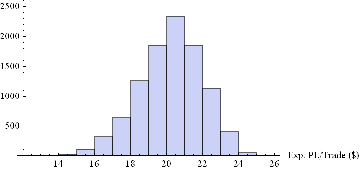
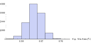
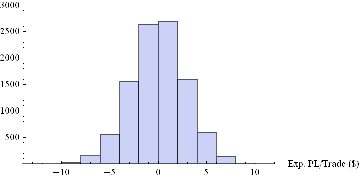
Now we can generate a random sample of 10, 000 simulation runs and plot a histogram of the Win Rates, using, for example, ES on 5-min bars, with a PT of 2 ticks and SL of – 20 ticks, assuming annual volatility of 15 %.
Histogram[Table[GenWinRate[1900,0.15,5,2,-20,0.25,12.50,3][[2]],{i,10000}],10,AxesLabel{“Exp. Win Rate (%)”}]

Histogram[Table[GenWinRate[1900,0.15,5,2,-20,0.25,12.50,3][[1]],{i,10000}],10,AxesLabel{“Exp. PL/Trade ($)”}]
Next we can do the same for the Extreme Value Distribution version of the model.
GenWinRateExtreme[currentPrice_,annualVolatility_,BarSizeMins_, nTicksPT_, nTicksSL_,minMove_, tickValue_, costContract_]:=Module[{ nMinsPerDay, periodVolatility, randObs, tgtReturn, slReturn,tgtDollar, slDollar, alpha, beta,nWins,nLosses, perTradePL, probWin, probLoss, winRate, expWinDollar, expLossDollar, expProfit},
nMinsPerDay = 250*6.5*60;
periodVolatility = annualVolatility / Sqrt[nMinsPerDay/BarSizeMins];
beta = Sqrt[6]*periodVolatility / Pi;
alpha=-EulerGamma*beta;
tgtReturn=nTicksPT*minMove/currentPrice;tgtDollar = nTicksPT * tickValue;
slReturn = nTicksSL*minMove/currentPrice;
slDollar=nTicksSL*tickValue;
randObs=RandomVariate[ExtremeValueDistribution[alpha, beta],10^3];
nWins=Count[randObs,x_/;x>=tgtReturn];
nLosses=Count[randObs,x_/;xslReturn];
winRate=nWins/(nWins+nLosses)//N;
perTradePL=(nWins*tgtDollar+nLosses*slDollar)/(nWins+nLosses);{perTradePL,winRate}]
Histogram[Table[GenWinRateExtreme[1900,0.15,5,2,-10,0.25,12.50,3][[2]],{i,10000}],10,AxesLabel{“Exp. Win Rate (%)”}]
Histogram[Table[GenWinRateExtreme[1900,0.15,5,2,-10,0.25,12.50,3][[1]],{i,10000}],10,AxesLabel{“Exp. PL/Trade ($)”}]
The key conclusions from this analysis are:
With all the marvelous new functionality that we have come to expect with each release, it is sometimes challenging to maintain a grasp on what the Wolfram language encompasses currently, let alone imagine what it might look like in another ten years. Indeed, the pace of development appears to be accelerating, rather than slowing down. However, I predict that the “problem” is soon about to get much, much worse. What I foresee is a step change in the pace of development of the Wolfram Language that will produce in days and weeks, or perhaps even hours and minutes, functionality might currently take months or years to develop. So obvious and clear cut is this development that I have hesitated to write about it, concerned that I am simply stating something that is blindingly obvious to everyone. But I have yet to see it even hinted at by others, including Wolfram. I find this surprising, because it will revolutionize the way in which not only the Wolfram language is developed in future, but in all likelihood programming and language development in general.
The key to this paradigm shift lies in the following unremarkable-looking WL function WolframLanguageData[], which gives a list of all Wolfram Language symbols and their properties. So, for example, we have:
WolframLanguageData[“SampleEntities”]
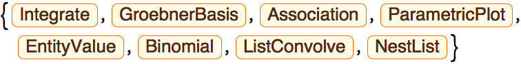
This means we can treat WL language constructs as objects, query their properties and apply functions to them, such as, for example:
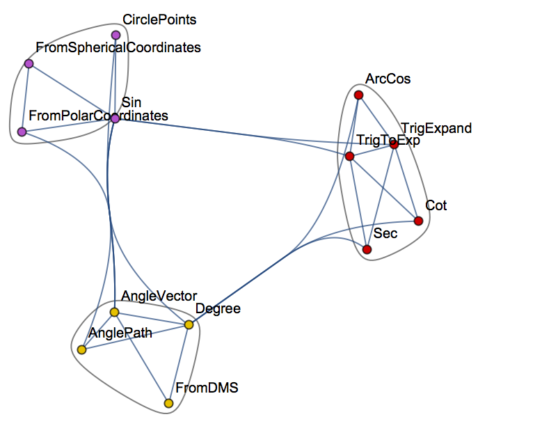
WolframLanguageData[“Cos”, “RelationshipCommunityGraph”]
In other words, the WL gives us the ability to traverse the entirety of the WL itself, combining WL objects into expressions, or programs.
This process is one definition of the term “Metaprogramming”. What I am suggesting is that in future, much of the heavy lifting will be carried out, not by developers, but by WL programs designed to produce code by metaprogramming. If successful, such an approach could streamline and accelerate the development process, speeding it up many times and, eventually, opening up areas of development that are currently beyond our imagination (and, possibly, our comprehension). So how does one build a metaprogramming system? This is where I should hand off to a computer scientist (and will happily do so as soon as one steps forward to take up the discussion). But here is a simple outline of one approach.
The principal tool one might use for such a task is genetic programming:
WikipediaData[“Genetic Programming”]
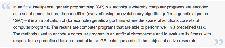
Actually, one can take issue with this explanation on several fronts, in particular the suggestion that GP is used primarily as a means of generating a computer program for performing a predefined task. That may certainly be the case, but need not be. Leaving that aside, the idea in simple terms is that we write a program that traverses the WL structure in some way, splicing together language objects to create a WL program that “does something”. That “something” may be a predefined task and indeed this would be a great place to start: to write a GP Metaprogramming system that creates programs that replicate the functionality of existing WL functions. Most of the generated programs would likely be uninteresting, slower versions of existing functions; but it is conceivable, I suppose, that some of the results might be of academic interest, or indicate a potentially faster computation method, perhaps. However, the point of the exercise is to get started on the Metaprogramming project, with a simple(ish) task with very clear, pre-defined goals and producing results that are easily tested. In this case the “objective function” is a comparison of results produced by the inbuilt WL functions vs the GP-generated functions, across some selected domain for the inputs. I glossed over the question of exactly how one “traverses the WL structure” for good reason: I feel quite sure that there must have been tremendous advances in the theory of how to do this in the last 50 years. But just to get the ball rolling, one could, for instance, operate a dual search, with a local search evaluating all of the functions closely connected to the (randomly chosen) starting function (WL object, while a second “long distance” search routine jumps randomly to a group of functions some specified number of steps away from the starting function. [At this point I envisage the computer scientists rolling their eyes and muttering “doesn’t this idiot know about the {fill in the blank} theorem about efficient domain search algorithms?”]. Anyway, to continue.
The initial exercise described above is about the mechanics of the process rather that the outcome. The second stage is much more challenging, as the goal is to develop new functionality, rather than simply to replicate what already exists. It would entail defining a much more complex objective function, as well as perhaps some constraints on program size, the number and types of WL objects used, etc. An interesting exercise, for example, would be to try to develop a metaprogramming system capable of winning the Wolfram One-Liner contest. Here, one might characterize the objective function as “something interesting and surprising”, and we would impose a tight constraint on the length of programs generated by the metaprogramming system to a single line of code. What is “interesting and surprising”? To be defined – that’s a central part of the challenge. But, in principle, I suppose one might try to train a neural network to classify whether or not a result is “interesting” based on the results of prior one-liner competitions.
From there, it’s on to the hard stuff: designing metaprogramming systems to produce WL programs of arbitrary length and complexity to do “interesting stuff” in a specific domain. That “interesting stuff” could be a more efficient approximation for a certain type of computation, a new algorithm for detecting certain patterns, or coming up with some completely novel formula or computational concept.
Obviously one faces huge challenges with this undertaking; but the potential rewards are enormous in terms of accelerating the pace of language development and discovery. It is a fascinating area for R&D, one that the WL is ideally situated to exploit. Indeed, I would be mightily surprised to learn that there is not already a team engaged on just such research at Wolfram. If so, perhaps one of them could comment here?