
Correlation Analysis of Emerging Markets


QUANTITATIVE RESEARCH AND TRADING
The latest theories, models and investment strategies in quantitative research and trading

In a previous post, Copulas in Risk Management, I covered in detail the theory and applications of copulas in the area of risk management, pointing out the potential benefits of the approach and how it could be used to improve estimates of Value-at-Risk by incorporating important empirical features of asset processes, such as asymmetric correlation and heavy tails.
In this post I will take a very different tack, demonstrating how copula models have potential applications in trading strategy design, in particular in pairs trading and statistical arbitrage strategies.
This is not a new concept – in fact the idea occurred to me (and others) many years ago, when copulas began to be widely adopted in financial engineering, risk management and credit derivatives modeling. But it remains relatively under-explored compared to more traditional techniques in this field. Fresh research suggests that it may be a useful adjunct to the more common methods applied in pairs trading, and may even be a more robust methodology altogether, as we shall see.
http://jonathankinlay.com/2017/01/copulas-risk-management/
http://jonathankinlay.com/2015/02/statistical-arbitrage-using-kalman-filter/
http://jonathankinlay.com/2015/02/developing-statistical-arbitrage-strategies-using-cointegration/
Over the last twenty five years significant advances have been made in the theory of asset processes and there now exist a variety of mathematical models, many of them computationally tractable, that provide a reasonable representation of their defining characteristics.
While the Geometric Brownian Motion model remains a staple of stochastic calculus theory, it is no longer the only game in town. Other models, many more sophisticated, have been developed to address the shortcomings in the original. There now exist models that provide a good explanation of some of the key characteristics of asset processes that lie beyond the scope of models couched in a simple Gaussian framework. Features such as mean reversion, long memory, stochastic volatility, jumps and heavy tails are now readily handled by these more advanced tools.
In this post I review a critical selection of asset process models that belong in every financial engineer’s toolbox, point out their key features and limitations and give examples of some of their applications.

One of the most widely used risk measures is the Value-at-Risk, defined as the expected loss on a portfolio at a specified confidence level. In other words, VaR is a percentile of a loss distribution.
But despite its popularity VaR suffers from well-known limitations: its tendency to underestimate the risk in the (left) tail of the loss distribution and its failure to capture the dynamics of correlation between portfolio components or nonlinearities in the risk characteristics of the underlying assets.
One method of seeking to address these shortcomings is discussed in a previous post Copulas in Risk Management. Another approach known as Conditional Value at Risk (CVaR), which seeks to focus on tail risk, is the subject of this post. We look at how to estimate Conditional Value at Risk in both Gaussian and non-Gaussian frameworks, incorporating loss distributions with heavy tails and show how to apply the concept in the context of nonlinear time series models such as GARCH.


Text and sentiment analysis has become a very popular topic in quantitative research over the last decade, with applications ranging from market research and political science, to e-commerce. In this post I am going to outline an approach to the subject, together with some core techniques, that have applications in investment strategy.
In the early days of the developing field of market sentiment analysis, the supply of machine readable content was limited to mainstream providers of financial news such as Reuters or Bloomberg. Over time this has changed with the entry of new competitors in the provision of machine readable news, including, for example, Ravenpack or more recent arrivals like Accern. Providers often seek to sell not only the raw news feed service, but also their own proprietary sentiment indicators that are claimed to provide additional insight into how individual stocks, market sectors, or the overall market are likely to react to news. There is now what appears to be a cottage industry producing white papers seeking to demonstrate the value of these services, often accompanied by some impressive pro-forma performance statistics for the accompanying strategies, which include long-only, long/short, market neutral and statistical arbitrage.
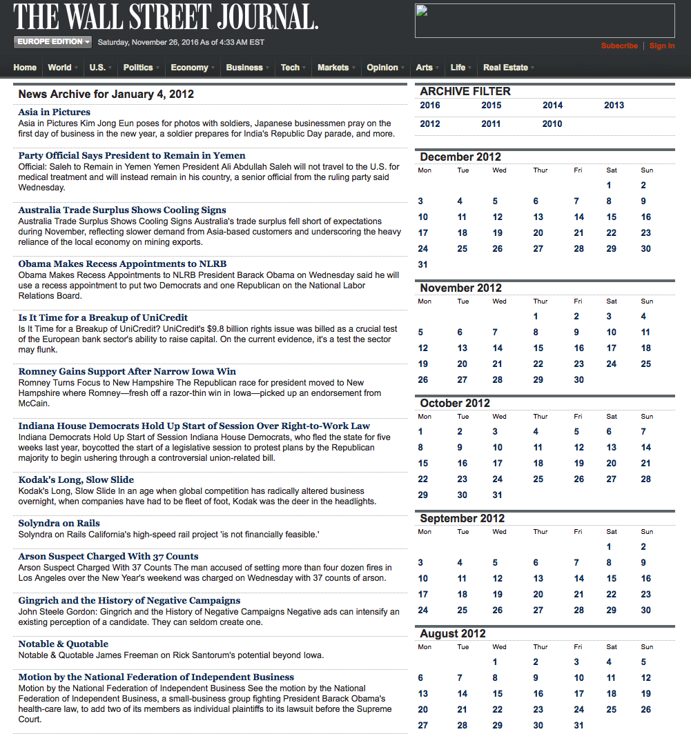
For the purpose of demonstration I intend to forego the blandishments of these services, although many are no doubt are excellent, since the reader is perhaps unlikely to have access to them. Instead, in what follows I will focus on a single news source, albeit a highly regarded one: the Wall Street Journal. This is, of course, a simplification intended for illustrative purposes only – in practice one would need to use a wide variety of news sources and perhaps subscribe to a machine readable news feed service. But similar principles and techniques can be applied to any number of news feeds or online sites.
We are going to access the Journal’s online archive, which presents daily news items in a convenient summary format, an example of which is shown below. The archive runs from the beginning of 2012 through to the current day, providing ample data for analysis. In what follows, I am going to make two important assumptions, neither of which is likely to be 100% accurate – but which will not detract too much from the validity of the research, I hope. The first assumption is that the news items shown in each daily archive were reported prior to the market open at 9:30 AM. This is likely to be true for the great majority of the stories, but there are no doubt important exceptions. Since we intend to treat the news content of each archive as antecedent to the market action during the corresponding trading session, exceptions are likely to introduce an element of look-ahead bias. The second assumption is that the archive for each day is shown in the form in which it would have appeared on the day in question. In reality, there are likely to have been revisions to some of the stories made subsequent to their initial publication. So, here too, we must allow for the possibility of look-ahead bias in the ensuing analysis.
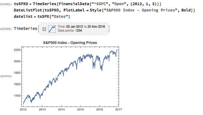
With those caveats out of the way, let’s proceed. We are going to be using broad market data for the S&P 500 index in the analysis to follow, so the first step is to download daily price series for the index. Note that we begin with daily opening prices, since we intend to illustrate the application of news sentiment analysis with a theoretical day-trading strategy that takes positions at the start of each trading session, exiting at market close.
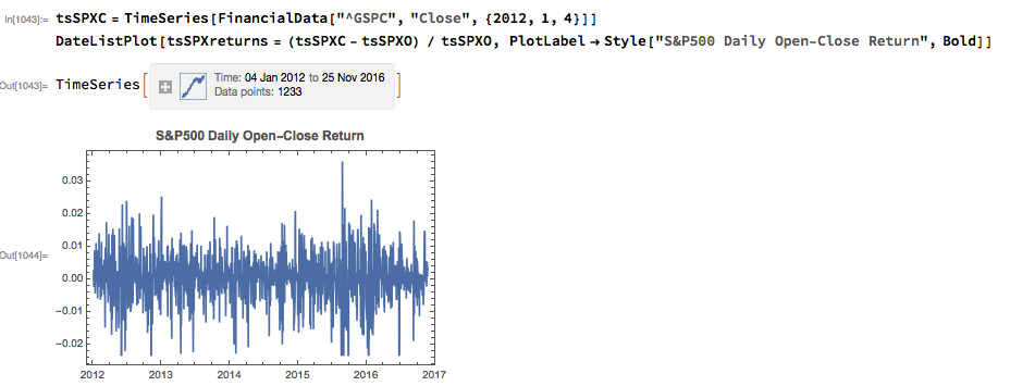
From there we calculate the intraday return in the index, from market open to close, as follows:
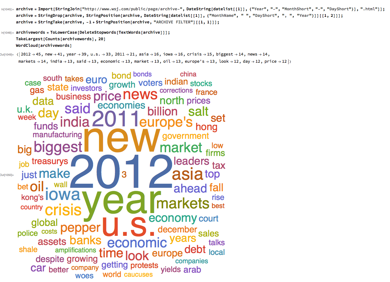
Next we turn to the task of reading the news archive and categorizing its content. Mathematica makes the importation of html pages very straightforward, and we can easily crop the raw text string to exclude page headers and footers. The approach I am going to take is to derive a sentiment indicator based on an analysis of the sentiment of each word in the daily archive. Before we can do that we must first convert the text into individuals words, stripping out standard stop-words such as “the” and “in” and converting all the text to lower case. Naturally one can take this pre-processing a great deal further, by identifying and separating out proper nouns, for example. Once the text processing stage is complete we can quickly summarize the content, for example by looking at the most common words, or by representing the entire archive in the form of a word cloud. Given that we are using the archive for the first business day of 2012, it is perhaps unsurprising that we find that “2012”, “new” and “year” feature so prominently!
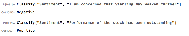
The subject of sentiment analysis is a complex one and I only touch on it here. For those interested in the subject I can recommend The Text Mining Handbook, by Feldman and Sanger, which is a standard work on the topic. Here I am going to employ a machine learning classifier provided with Mathematica 11. It is not terribly sophisticated (or, at least, has not been developed with financial applications especially in mind), but will serve for the purposes of this article. For those unfamiliar with the functionality, the operation of the sentiment classification algorithm is straightforward enough. For instance:
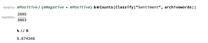
We apply the algorithm to classify each word in the daily news archive and arrive at a sentiment indicator based on the proportion of words that are classified as “positive”. The sentiment reading for the archive for Jan-3, 2012, for example, turns out to be 67.4%:
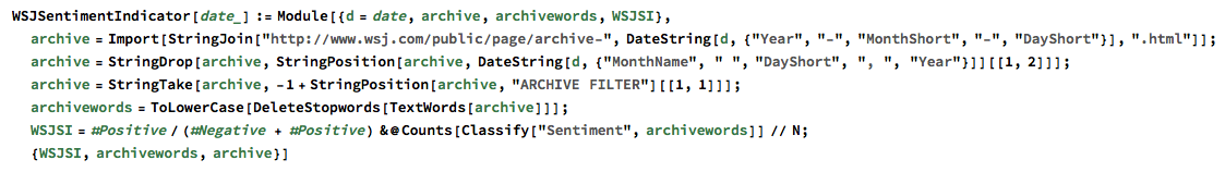
We can automate the process of classifying the entire WSJ archive with just a few lines of code, producing a time series for the daily sentiment indicator, which has an average daily value of 68.5% – the WSJ crowd tends to be bullish, clearly! Note how the 60-day moving average of the indicator rises steadily over the period from 2012 through Q1 2015, then abruptly reverses direction, declining steadily thereafter – even somewhat precipitously towards the end of 2016.

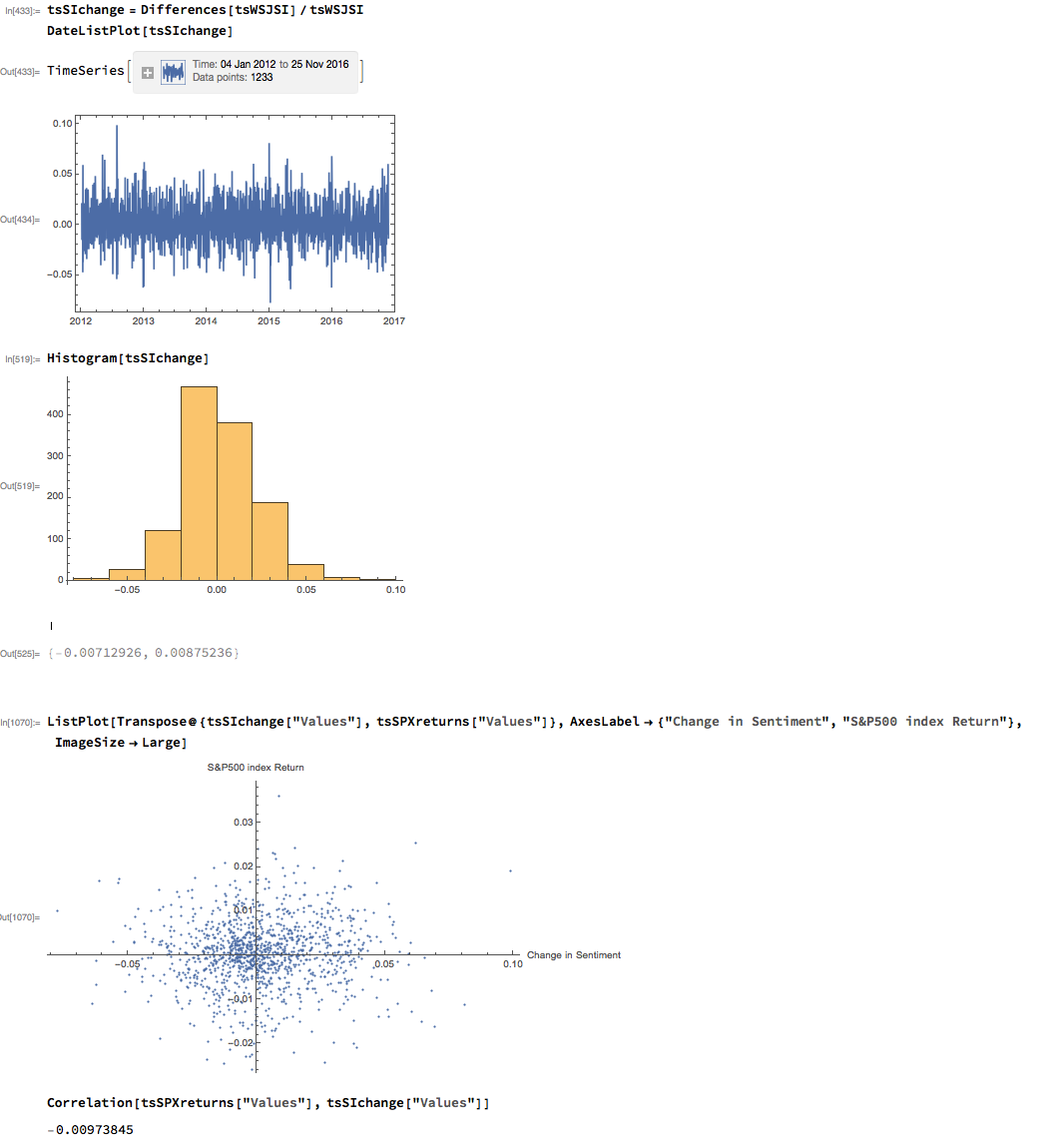
As with most data series in investment research, we are less interested in the level of a variable, such as a stock price, than we are in the changes in level. So the next step is to calculate the daily percentage change in the sentiment indicator and examine the correlation with the corresponding intraday return in the S&P 500 Index. At first glance our sentiment indicator appears to have very little predictive power – the correlation between indicator changes and market returns is negligibly small overall – but we shall later see that this is not the last word.
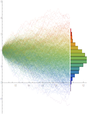
Thus far the results appear discouraging; but as is often the case with this type of analysis we need to look more closely at the conditional distribution of returns. Specifically, we will examine the conditional distribution of S&P 500 Index returns when changes in the sentiment index are in the upper and lower quantiles of the distribution. This will enable us to isolate the impact of changes in market sentiment at times when the swings in sentiment are strongest. In the analysis below, we begin by examining the upper and lower third of the distribution of changes in sentiment:
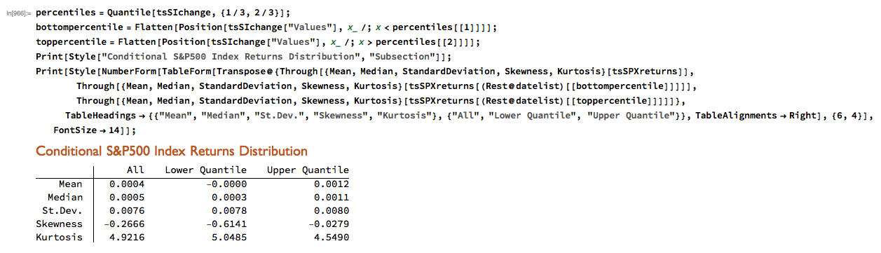
The analysis makes clear that the distribution of S&P 500 Index returns is very different on days when the change in market sentiment is large and positive vs. large and negative. The difference is not just limited to the first moment of the conditional distribution, where the difference in the mean return is large and statistically significant, but also in the third moment. The much larger, negative skewness means that there is a greater likelihood of a large decline in the market on days in which there is a sizable drop in market sentiment, than on days in which sentiment significantly improves. In other words, the influence of market sentiment changes is manifest chiefly through the mean and skewness of the conditional distributions of market returns.
We can capitalize on these effects using a simple trading strategy in which we increase the capital allocated to a long-SPX position on days when market sentiment improves, while reducing exposure on days when market sentiment falls. We increase the allocation by a factor – designated the leverage factor – on days when the change in the sentiment indicator is in the upper 1/3 of the distribution, while reducing the allocation by 1/leveragefactor on days when the change in the sentiment indicator falls in lower 1/3 of the distribution. The allocation on other days is 100%. The analysis runs as follows:

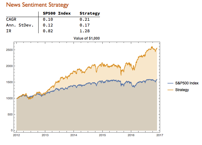
It turns out that, using a leverage factor of 2.0, we can increase the CAGR from 10% to 21% over the period from 2012-2016 using the conditional distribution approach. This performance enhancement comes at a cost, since the annual volatility of the news sentiment strategy is 17% compared to only 12% for the long-only strategy. However, the overall net result is positive, since the risk-adjusted rate of return increases from 0.82 to 1.28.
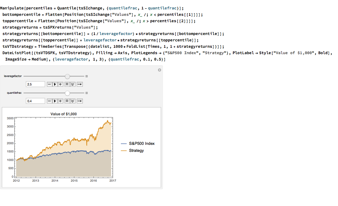
We can explore the robustness of the result, comparing different quantile selections and leverage factors using Mathematica’s interactive Manipulate function:
We have seen that a simple market sentiment indicator can be created quite easily from publicly available news archives, using a standard machine learning sentiment classification algorithm. A market sentiment algorithm constructed using methods as straightforward as this appears to provide the capability to differentiate the conditional distribution of market returns on days when changes in market sentiment are significantly positive or negative. The differences in the higher moments of the conditional distribution appears to be as significant as the differences in the mean. In principle, we can use the insight provided by the sentiment indicator to enhance a long-only day-trading strategy, increasing leverage and allocation on days when changes to market sentiment are positive and reducing them on days when sentiment declines. The performance enhancements resulting from this approach appear to be significant.
Several caveats apply. The S&P 500 index is not tradable, of course, and it is not uncommon to find trading strategies that produce interesting theoretical results. In practice one would be obliged to implement the strategy using a tradable market proxy, such as a broad market ETF or futures contract. The strategy described here, which enters and exits positions daily, would incur substantial trading costs, that would be further exacerbated by the use of leverage.
Of course there are many other uses one can make of news data, in particular with firm-specific news and sentiment analytics, that fall outside the scope of this article. Hopefully, however, the methodology described here will provide a sign-post towards further, more practically useful research.
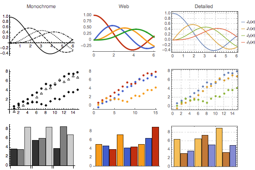
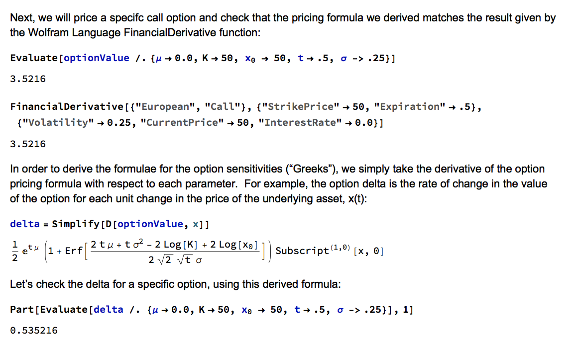
Wolfram Research introduced random processes in version 9 of Mathematica and for the first time users were able to tackle more complex modeling challenges such as those arising in stochastic calculus. The software’s capabilities in this area have grown and matured over the last two versions to a point where it is now feasible to teach stochastic calculus and the fundamentals of financial engineering entirely within the framework of the Wolfram Language. In this post we take a lightening tour of some of the software’s core capabilities and give some examples of how it can be used to create the building blocks required for a complete exposition of the theory behind modern finance.
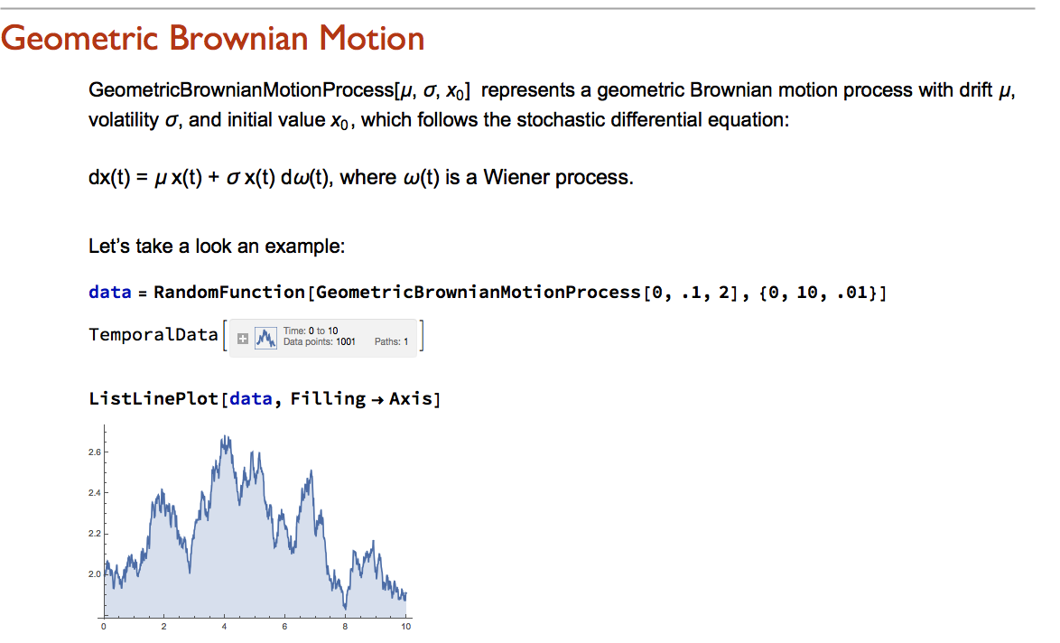
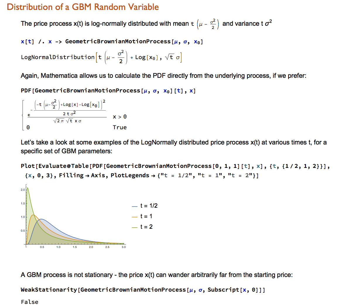
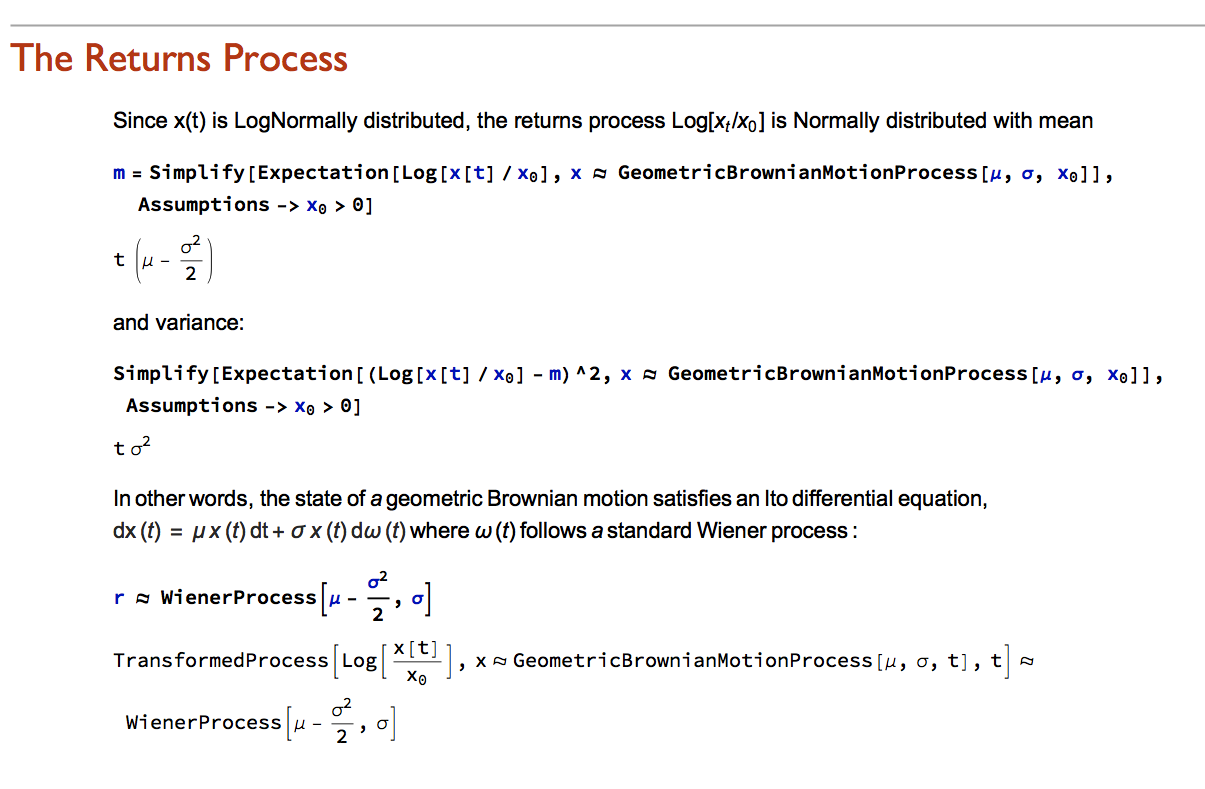


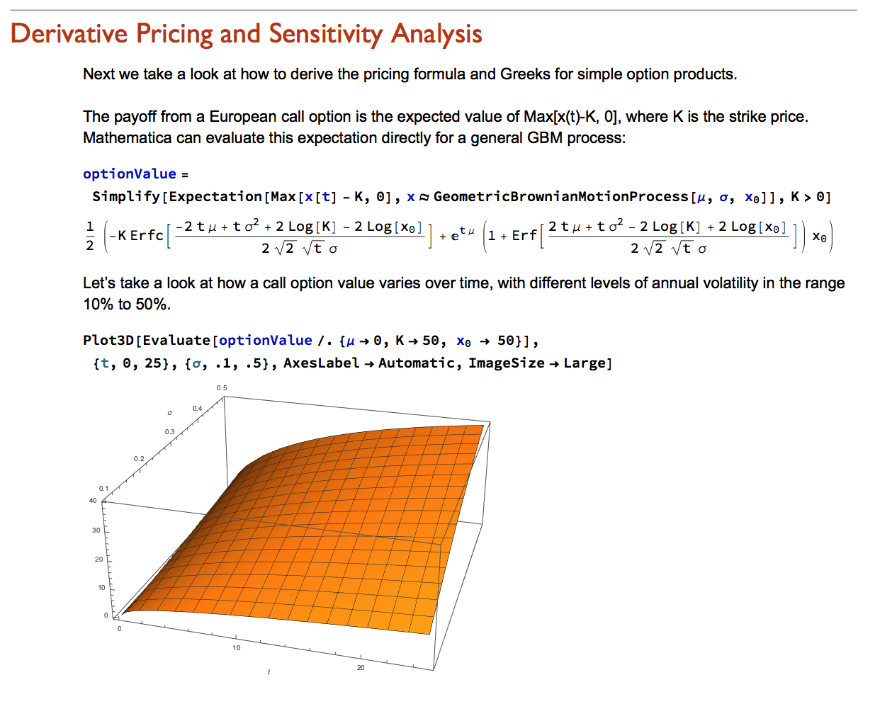
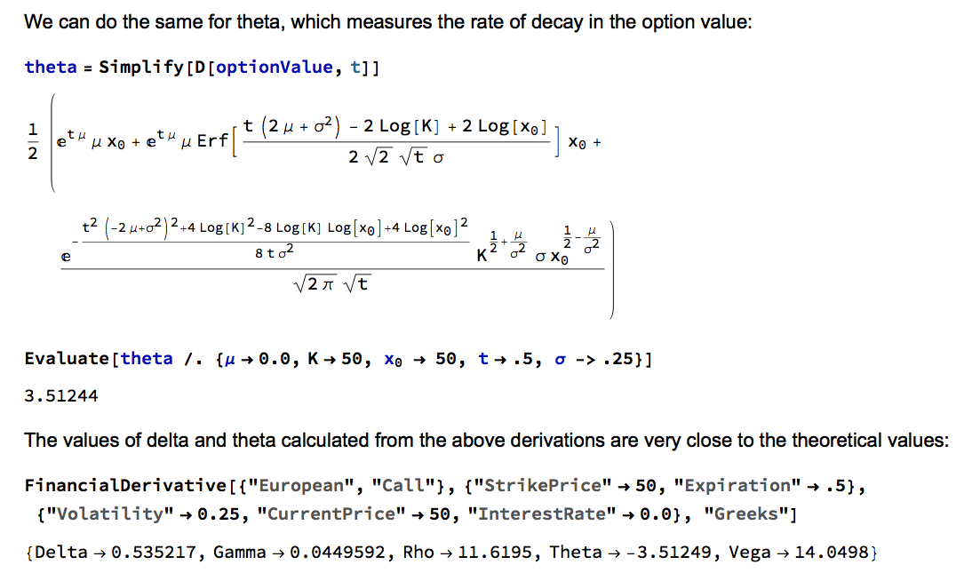
Financial Engineering has long been a staple application of Mathematica, an area in which is capabilities in symbolic logic stand out. But earlier versions of the software lacked the ability to work with Ito calculus and model stochastic processes, leaving the user to fill in the gaps by other means. All that changed in version 9 and it is now possible to provide the complete framework of modern financial theory within the context of the Wolfram Language.
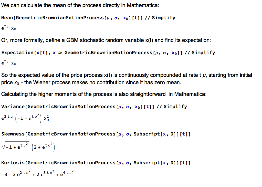
The advantages of this approach are considerable. The capabilities of the language make it easy to provide interactive examples to illustrate theoretical concepts and develop the student’s understanding of them through experimentation. Furthermore, the student is not limited merely to learning and applying complex formulae for derivative pricing and risk, but can fairly easily derive the results for themselves. As a consequence, a course in stochastic calculus taught using Mathematica can be broader in scope and go deeper into the theory than is typically the case, while at the same time reinforcing understanding and learning by practical example and experimentation.


Precious metals have been in free-fall for several years, as a consequence of the Fed’s actions to stimulate the economy that have also had the effect of goosing the equity and fixed income markets. All that changed towards the end of 2015, as the Fed moved to a tightening posture. So far, 2016 has been a banner year for metal, with spot prices for platinum, gold and silver up 26%, 28% and 44% respectively.
So what are the prospects for metals through the end of the year? We take a shot at predicting the outcome, from a quantitative perspective.

![]()
Source: Wolfram Alpha. Spot silver prices are scaled x100
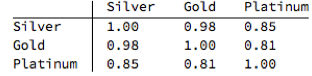
One of the key characteristics of metals is the very high levels of price-correlation between them. Over the period under investigation, Jan 2012 to Aug 2016, the estimated correlation coefficients are as follows:
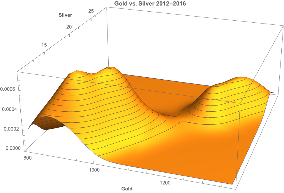
A plot of the join density of spot gold and silver prices indicates low- and high-price regimes in which the metals display similar levels of linear correlation.

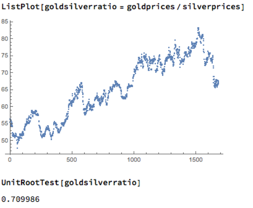
Levels of correlation that are consistently as high as this over extended periods of time are fairly unusual in financial markets and this presents a potential trading opportunity. One common approach is to use the ratios of metal prices as a trading signal. However, taking the ratio of gold to silver spot prices as an example, a plot of the series demonstrates that it is highly unstable and susceptible to long term trends.
A more formal statistical test fails to reject the null hypothesis of a unit root. In simple terms, this means we cannot reliably distinguish between the gold/silver price ratio and a random walk.
Along similar lines, we might consider the difference in log prices of the series. If this proved to be stationary then the log-price series would be cointegrated order 1 and we could build a standard pairs trading model to buy or sell the spread when prices become too far unaligned. However, we find once again that the log-price difference can wander arbitrarily far from its mean, and we are unable to reject the null hypothesis that the series contains a unit root.

We can hope to do better with a standard linear model, regressing spot silver prices against spot gold prices. The fit of the best linear model is very good, with an R-sq of over 96%:
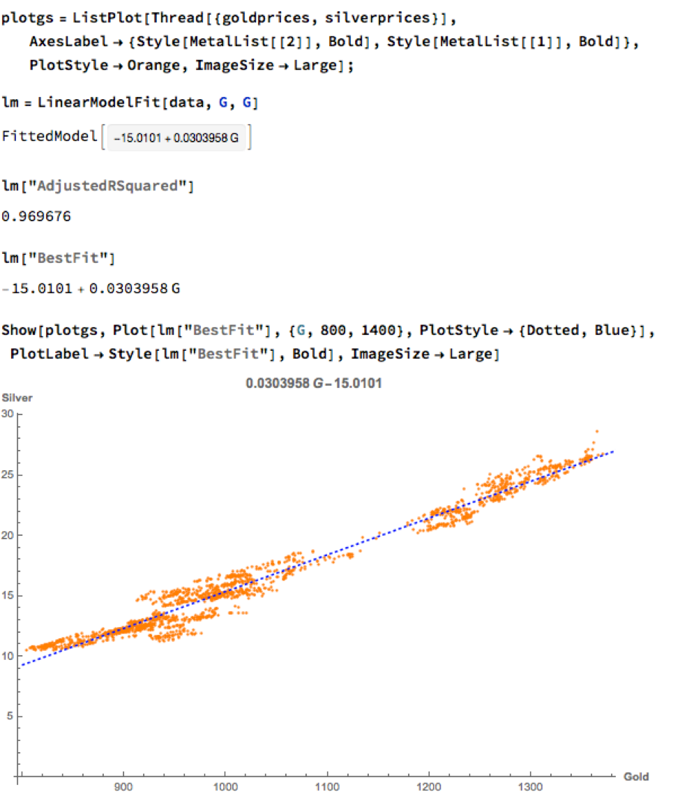
A trader might look to exploit the correlation relationship by selling silver when its market price is greater than the value estimated by the model (and buying when the model price exceeds the market price). Typically the spread is bought or sold when the log-price differential exceeds a threshold level that is set at twice the standard deviation of the price-difference series. The threshold levels derive from the assumption of Normality, which in fact does not apply here, as we can see from an examination of the residuals of the linear model:
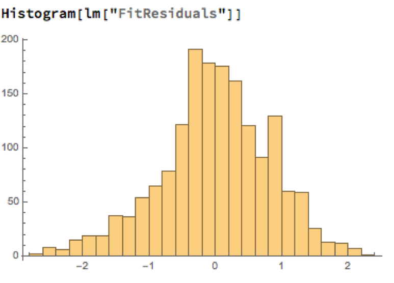
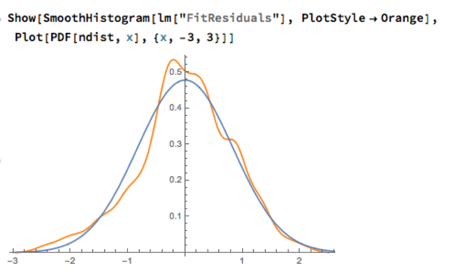
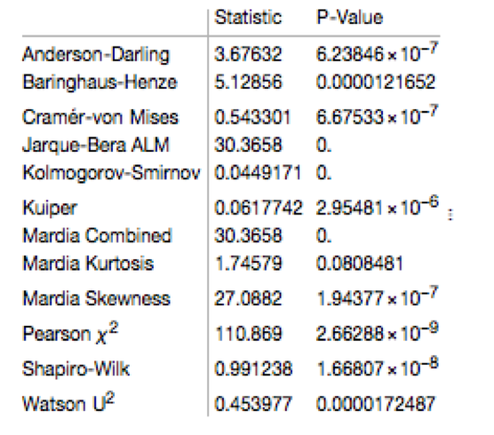
Given the evident lack of fit, especially in the left tail of the distribution, it is unsurprising that all of the formal statistical tests for Normality easily reject the null hypothesis:
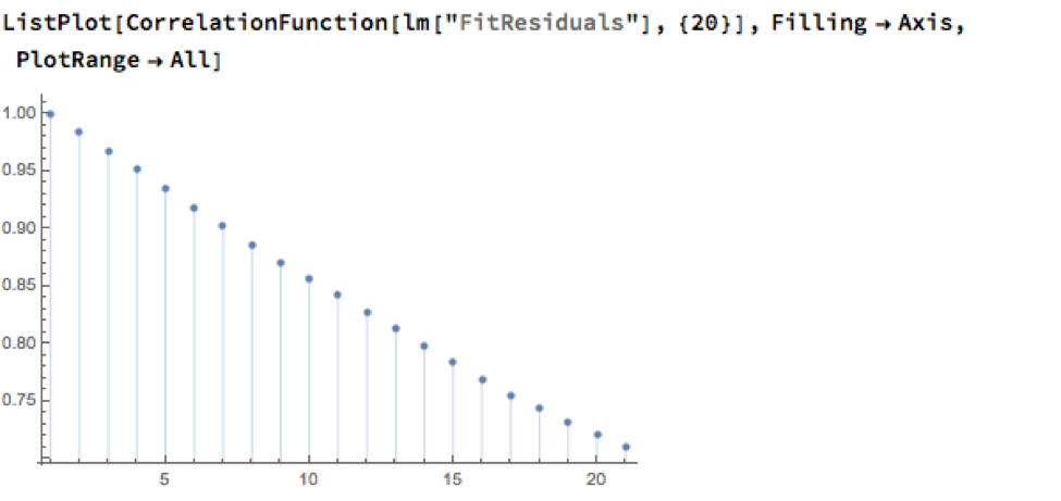
However, Normality, or the lack of it, is not the issue here: one could just as easily set the 2.5% and 97.5% percentiles of the empirical distribution as trade entry points. The real problem with the linear model is that it fails to take into account the time dependency in the price series. An examination of the residual autocorrelations reveals significant patterning, indicating that the model tends to under-or over-estimate the spot price of silver for long periods of time:
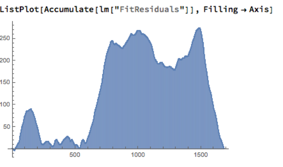
As the following chart shows, the cumulative difference between model and market prices can become very large indeed. A trader risks going bust waiting for the market to revert to model prices.
How does one remedy this? The shortcoming of the simple linear model is that, while it captures the interdependency between the price series very well, it fails to factor in the time dependency of the series. What is required is a model that will account for both features.
Rather than modeling the metal prices individually, or in pairs, we instead adopt a multivariate vector autoregression approach, modeling all three spot price processes together. The essence of the idea is that spot prices in each metal may be influenced, not only by historical values of the series, but also potentially by current and lagged prices of the other two metals.
Before proceeding we divide the data into two parts: an in-sample data set comprising data from 2012 to the end of 2015 and an out-of-sample period running from Jan-Aug 2016, which we use for model testing purposes. In what follows, I make the simplifying assumption that a vector autoregressive moving average process of order (1, 1) will suffice for modeling purposes, although in practice one would go through a procedure to test a wide spectrum of possible models incorporating moving average and autoregressive terms of varying dimensions.
In any event, our simplified VAR model is estimated as follows:

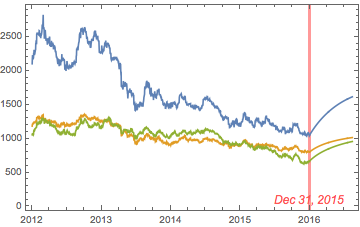
The chart below combines the actual, in-sample data from 2012-2015, together with the out-of-sample forecasts for each spot metal from January 2016.
![]()
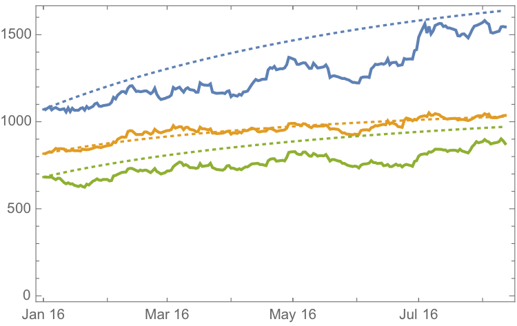
It is clear that the model projects a recovery in spot metal prices from the end of 2015. How did the forecasts turn out? In the chart below we compare the actual spot prices with the model forecasts, over the period from Jan to Aug 2016.
![]()
The actual and forecast percentage change in the spot metal prices over the out-of-sample period are as follows:
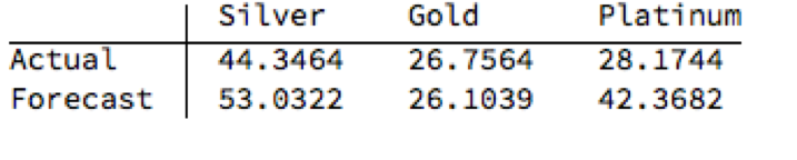
The VAR model does a good job of forecasting the strong upward trend in metal prices over the first eight months of 2016. It performs exceptionally well in its forecast of gold prices, although its forecasts for silver and platinum are somewhat over-optimistic. Nevertheless, investors would have made money taking a long position in any of the metals on the basis of the model projections.
Another way to apply the model would be to implement a relative value trade, based on the model’s forecast that silver would outperform gold and platinum. Indeed, despite the model’s forecast of silver prices turning out to be over-optimistic, a relative value trade in silver vs. gold or platinum would have performed well: silver gained 44% in the period form Jan-Aug 2016, compared to only 26% for gold and 28% for platinum. A relative value trade entailing a purchase of silver and simultaneous sale of gold or platinum would have produced a gross return of 17% and 15% respectively.
A second relative value trade indicated by the model forecasts, buying platinum and selling gold, would have turned out less successfully, producing a gross return of less than 2%. We will examine the reasons for this in the next section.
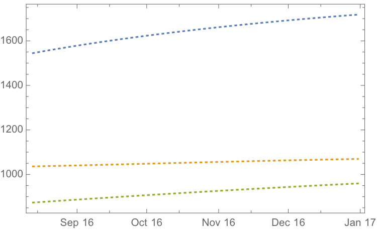
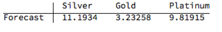
If we re-estimate the VAR model using all of the the available data through mid-Aug 2016 and project metal prices through the end of the year, the outcome is as follows:
![]()
While the positive trend in all three metals is forecast to continue, the new model (which incorporates the latest data) anticipates lower percentage rates of appreciation going forward:
Once again, the model predicts higher rates of appreciation for both silver and platinum relative to gold. So investors have the option to take a relative value trade, hedging a long position in silver or platinum with a short position in gold. While the forecasts for all three metals appear reasonable, the projections for platinum strike me as the least plausible.
The reason is that the major applications of platinum are industrial, most often as a catalyst: the metal is used as a catalytic converter in automobiles and in the chemical process of converting naphthas into higher-octane gasolines. Although gold is also used in some industrial applications, its demand is not so driven by industrial uses. Consequently, during periods of sustained economic stability and growth, the price of platinum tends to be as much as twice the price of gold, whereas during periods of economic uncertainty, the price of platinum tends to decrease due to reduced industrial demand, falling below the price of gold. Gold prices are more stable in slow economic times, as gold is considered a safe haven.
This is the most likely explanation of why the gold-platinum relative value trade has not worked out as expected hitherto and is perhaps unlikely to do so in the months ahead, as the slowdown in the global economy continues.
We have shown that simple models of the ratio or differential in the prices of precious metals are unlikely to provide a sound basis for forecasting or trading, due to non-stationarity and/or temporal dependencies in the residuals from such models.
On the other hand, a vector autoregression model that models all three price processes simultaneously, allowing both cross correlations and autocorrelations to be captured, performs extremely well in terms of forecast accuracy in out-of-sample tests over the period from Jan-Aug 2016.
Looking ahead over the remainder of the year, our updated VAR model predicts a continuation of the price appreciation, albeit at a slower rate, with silver and platinum expected to continue outpacing gold. There are reasons to doubt whether the appreciation of platinum relative to gold will materialize, however, due to falling industrial demand as the global economy cools.