Optimal Mean-Reversion Strategies

Consider a financial asset whose price, Xt​, follows a mean-reverting stochastic process. A common model for mean reversion is the Ornstein-Uhlenbeck (OU) process, defined by the stochastic differential equation (SDE):

The trader aims to maximize the expected cumulative profit from trading this asset over a finite horizon, subject to transaction costs. The trader’s control is the rate of buying or selling the asset, denoted by ut​, at time t.

To find the optimal trading strategy, we frame this as a stochastic control problem. The value function,V(t,Xt​), represents the maximum expected profit from time t to the end of the trading horizon, given the current price level Xt​. The HJB equation for this problem is:

where C(ut​) represents the cost of trading, which can depend on the rate of trading ut​. The term ut​(Xt​−C(ut​)) captures the profit from trading, adjusted for transaction costs.

Boundary and Terminal Conditions: Specify terminal conditions for V(T,XT​), where T is the end of the trading horizon, and boundary conditions for V(t,Xt​) based on the problem setup.

Solve the HJB Equation: The solution involves finding the function V(t,Xt​) and the control policy ut∗​ that maximizes the HJB equation. This typically requires numerical methods, especially for complex cost functions or when closed-form solutions are not feasible.

Interpret the Optimal Policy: The optimal control ut∗​ derived from solving the HJB equation indicates the optimal rate of trading (buying or selling) at any time t and price level Xt​, considering the mean-reverting nature of the price and the impact of transaction costs.

No-Trade Zones: The presence of transaction costs often leads to the creation of no-trade zones in the optimal policy, where the expected benefit from trading does not outweigh the costs.

Mean-Reversion Exploitation: The optimal strategy exploits mean reversion by adjusting the trading rate based on the deviation of the current price from the mean level, μ.

The Lipton & Lopez de Marcos Paper

“A Closed-form Solution for Optimal Mean-reverting Trading Strategies” contributes significantly to the literature on optimal trading strategies for mean-reverting instruments. The paper focuses on deriving optimal trading strategies that maximize the Sharpe Ratio by solving the Hamilton-Jacobi-Bellman equation associated with the problem. It outlines a method that relies on solving a Fredholm integral equation to determine the optimal trading levels, taking into account transaction costs.

The paper begins by discussing the relevance of mean-reverting trading strategies across various markets, particularly emphasizing the energy market’s suitability for such strategies. It acknowledges the practical challenges and limitations of previous analytical results, mainly asymptotic and applicable to perpetual trading strategies, and highlights the novelty of addressing finite maturity strategies.

A key contribution of the paper is the development of an explicit formula for the Sharpe ratio in terms of stop-loss and take-profit levels, which allows traders to deploy tactical execution algorithms for optimal strategy performance under different market regimes. The methodology involves calibrating the Ornstein-Uhlenbeck process to market prices and optimizing the Sharpe ratio with respect to the defined levels. The authors present numerical results that illustrate the Sharpe ratio as a function of these levels for various parameters and discuss the implications of their findings for liquidity providers and statistical arbitrage traders.

The paper also reviews traditional approaches to similar problems, including the use of renewal theory and linear transaction costs, and compares these with its analytical framework. It concludes that its method provides a valuable tool for liquidity providers and traders to optimally execute their strategies, with practical applications beyond theoretical interest.

The authors use the path integral method to understand the behavior of their solutions, providing an alternative treatment to linear transaction costs that results in a determination of critical boundaries for trading. This approach is distinct in its use of direct solving methods for the Fredholm equation and adjusting the trading thresholds through a numerical method until a matching condition is met.

This research not only advances the understanding of optimal trading rules for mean-reverting strategies but also offers practical guidance for traders and liquidity providers in implementing these strategies effectively.

A Practical Application of Regime Switching Models to Pairs Trading

In the previous post I outlined some of the available techniques used for modeling market states.  The following is an illustration of how these techniques can be applied in practice.    You can download this post in pdf format here.

SSALGOTRADING AD

The chart below shows the daily compounded returns for a single pair in an ETF statistical arbitrage strategy, back-tested over a 1-year period from April 2010 to March 2011.

The idea is to examine the characteristics of the returns process and assess its predictability.

Pairs Trading

The initial impression given by the analytics plots of daily returns, shown in Fig 2 below, is that the process may be somewhat predictable, given what appears to be a significant 1-order lag in the autocorrelation spectrum.  We also see evidence of the
customary non-Gaussian “fat-tailed” distribution in the error process.

Regime Switching

An initial attempt to fit a standard Auto-Regressive Moving Average ARMA(1,0,1) model  yields disappointing results, with an unadjusted  model R-squared of only 7% (see model output in Appendix 1)

However, by fitting a 2-state Markov model we are able to explain as much as 65% in the variation in the returns process (see Appendix II).
The model estimates Markov Transition Probabilities as follows.

P(.|1)       P(.|2)

P(1|.)       0.93920      0.69781

P(2|.)     0.060802      0.30219

In other words, the process spends most of the time in State 1, switching to State 2 around once a month, as illustrated in Fig 3 below.

Markov model
In the first state, the  pairs model produces an expected daily return of around 65bp, with a standard deviation of similar magnitude.  In this state, the process also exhibits very significant auto-regressive and moving average features.

Regime 1:

Intercept                   0.00648     0.0009       7.2          0

AR1                            0.92569    0.01897   48.797        0

MA1                         -0.96264    0.02111   -45.601        0

Error Variance^(1/2)           0.00666     0.0007

In the second state, the pairs model  produces lower average returns, and with much greater variability, while the autoregressive and moving average terms are poorly determined.

Regime 2:

Intercept                    0.03554    0.04778    0.744    0.459

AR1                            0.79349    0.06418   12.364        0

MA1                         -0.76904    0.51601     -1.49   0.139

Error Variance^(1/2)           0.01819     0.0031

CONCLUSION
The analysis in Appendix II suggests that the residual process is stable and Gaussian.  In other words, the two-state Markov model is able to account for the non-Normality of the returns process and extract the salient autoregressive and moving average features in a way that makes economic sense.

How is this information useful?  Potentially in two ways:

(i)     If the market state can be forecast successfully, we can use that information to increase our capital allocation during periods when the process is predicted to be in State 1, and reduce the allocation at times when it is in State 2.

(ii)    By examining the timing of the Markov states and considering different features of the market during the contrasting periods, we might be able to identify additional explanatory factors that could be used to further enhance the trading model.

Markov model

Modeling Asset Volatility

I am planning a series of posts on the subject of asset volatility and option pricing and thought I would begin with a survey of some of the central ideas. The attached presentation on Modeling Asset Volatility sets out the foundation for a number of key concepts and the basis for the research to follow.

Perhaps the most important feature of volatility is that it is stochastic rather than constant, as envisioned in the Black Scholes framework.  The presentation addresses this issue by identifying some of the chief stylized facts about volatility processes and how they can be modelled.  Certain characteristics of volatility are well known to most analysts, such as, for instance, its tendency to “cluster” in periods of higher and lower volatility.  However, there are many other typical features that are less often rehearsed and these too are examined in the presentation.

Long Memory
For example, while it is true that GARCH models do a fine job of modeling the clustering effect  they typically fail to capture one of the most important features of volatility processes – long term serial autocorrelation.  In the typical GARCH model autocorrelations die away approximately exponentially, and historical events are seen to have little influence on the behaviour of the process very far into the future.  In volatility processes that is typically not the case, however:  autocorrelations die away very slowly and historical events may continue to affect the process many weeks, months or even years ahead.

Volatility Direction Prediction Accuracy

There are two immediate and very important consequences of this feature.  The first is that volatility processes will tend to trend over long periods – a characteristic of Black Noise or Fractionally Integrated processes, compared to the White Noise behavior that typically characterizes asset return processes.  Secondly, and again in contrast with asset return processes, volatility processes are inherently predictable, being conditioned to a significant degree on past behavior.  The presentation considers the fractional integration frameworks as a basis for modeling and forecasting volatility.

Mean Reversion vs. Momentum
A puzzling feature of much of the literature on volatility is that it tends to stress the mean-reverting behavior of volatility processes.  This appears to contradict the finding that volatility behaves as a reinforcing process, whose long-term serial autocorrelations create a tendency to trend.  This leads to one of the most important findings about asset processes in general, and volatility process in particular: i.e. that the assets processes are simultaneously trending and mean-reverting.  One way to understand this is to think of volatility, not as a single process, but as the superposition of two processes:  a long term process in the mean, which tends to reinforce and trend, around which there operates a second, transient process that has a tendency to produce short term spikes in volatility that decay very quickly.  In other words, a transient, mean reverting processes inter-linked with a momentum process in the mean.  The presentation discusses two-factor modeling concepts along these lines, and about which I will have more to say later.

SSALGOTRADING AD

Cointegration
One of the most striking developments in econometrics over the last thirty years, cointegration is now a principal weapon of choice routinely used by quantitative analysts to address research issues ranging from statistical arbitrage to portfolio construction and asset allocation.  Back in the late 1990’s I and a handful of other researchers realized that volatility processes exhibited very powerful cointegration tendencies that could be harnessed to create long-short volatility strategies, mirroring the approach much beloved by equity hedge fund managers.  In fact, this modeling technique provided the basis for the Caissa Capital volatility fund, which I founded in 2002.  The presentation examines characteristics of multivariate volatility processes and some of the ideas that have been proposed to model them, such as FIGARCH (fractionally-integrated GARCH).

Dispersion Dynamics
Finally, one topic that is not considered in the presentation, but on which I have spent much research effort in recent years, is the behavior of cross-sectional volatility processes, which I like to term dispersion.  It turns out that, like its univariate cousin, dispersion displays certain characteristics that in principle make it highly forecastable.  Given an appropriate model of dispersion dynamics, the question then becomes how to monetize efficiently the insight that such a model offers.  Again, I will have much more to say on this subject, in future.

Pairs Trading with Copulas

Introduction

In a previous post, Copulas in Risk Management, I covered in detail the theory and applications of copulas in the area of risk management, pointing out the potential benefits of the approach and how it could be used to improve estimates of Value-at-Risk by incorporating important empirical features of asset processes, such as asymmetric correlation and heavy tails.

In this post I will take a very different tack, demonstrating how copula models have potential applications in trading strategy design, in particular in pairs trading and statistical arbitrage strategies.

SSALGOTRADING AD

This is not a new concept – in fact the idea occurred to me (and others) many years ago, when copulas began to be widely adopted in financial engineering, risk management and credit derivatives modeling. But it remains relatively under-explored compared to more traditional techniques in this field. Fresh research suggests that it may be a useful adjunct to the more common methods applied in pairs trading, and may even be a more robust methodology altogether, as we shall see.

Recommended Background Reading

http://jonathankinlay.com/2017/01/copulas-risk-management/

http://jonathankinlay.com/2015/02/statistical-arbitrage-using-kalman-filter/

http://jonathankinlay.com/2015/02/developing-statistical-arbitrage-strategies-using-cointegration/


Pairs Trading with Copulas

Modeling Asset Processes

Introduction

Over the last twenty five years significant advances have been made in the theory of asset processes and there now exist a variety of mathematical models, many of them computationally tractable, that provide a reasonable representation of their defining characteristics.

SSALGOTRADING AD

While the Geometric Brownian Motion model remains a staple of stochastic calculus theory, it is no longer the only game in town.  Other models, many more sophisticated, have been developed to address the shortcomings in the original.  There now exist models that provide a good explanation of some of the key characteristics of asset processes that lie beyond the scope of models couched in a simple Gaussian framework. Features such as mean reversion, long memory, stochastic volatility,  jumps and heavy tails are now readily handled by these more advanced tools.

In this post I review a critical selection of asset process models that belong in every financial engineer’s toolbox, point out their key features and limitations and give examples of some of their applications.


Modeling Asset Processes

Is Internal Bar Strength A Random Walk? The Case of Exxon-Mobil

For those who prefer a little more rigor in their quantitative research, I can offer more a somewhat more substantive statistical argument in favor of the IBS indicator discussed in my previous post.

Specifically, we can show quite convincingly that the IBS process is stationary, a highly desirable property much sought-after in, for example, the construction of statistical arbitrage strategies.  Of course, by construction, the IBS is constrained to lie between the values of 0 and 1, so non-stationarity in the mean is highly unlikely.  But, conceivably, there could be some time dependency in the process or in its variance, for instance.  Then there is the further question as to whether the IBS indicator is mean-reverting, which would indicate that the underlying price process likewise has a tendency to mean revert.

Let’s take the IBS series for Exxon-Mobil (XOM) as an example to work with. I have computed the series from the beginning of 1990, and the first 100 values are shown in the plot below.


XOMIBS


Autocorrelation and Unit Root Tests

There appears to be little patterning in the process autocorrelations, and this is confirmed by formal statistical tests which fail to reject the null hypothesis that the first 20 autocorrelations are not, collectively, statistically significant.

XOMIBS Autocorrelations


XOMIBS acf test


SSALGOTRADING AD

Next we test for the presence of a unit root in the IBS process (highly unlikely, given its construction) and indeed, unsurprisingly, the null hypothesis of a unit root is roundly rejected by the Dickey-Fuller and Phillips-Perron tests.


XOMIBS Unit Root


Variance Ratio Tests

We next conduct a formal test to determine whether the IBS series follows a random walk.

The variance ratio test assesses the null hypothesis that a univariate time series y is a random walk. The null model is

y(t) = c + y(t–1) + e(t),

where c is a drift constant (assumed zero for the IBS series) and e(t) are uncorrelated innovations with zero mean.

  • When IID is false, the alternative is that the e(t) are correlated.
  • When IID is true, the alternative is that the e(t) are either dependent or not identically distributed (for example, heteroscedastic).


We test whether the XOM IBS series is a random walk using various step sizes and perform the test with and without the assumption that the innovations are independent and identically distributed.

Switching to Matlab, we proceed as follows:

q = [2 4 8 2 4 8];
flag = logical([1 1 1 0 0 0]);
[h,pValue,stat,cValue,ratio] = vratiotest(XOMIBS,’period’,q,’IID’,flag)

Here h is a vector of Boolean decisions for the tests, with length equal to the number of tests. Values of h equal to 1 indicate rejection of the random-walk null in favor of the alternative. Values of h equal to 0 indicate a failure to reject the random-walk null.

The variable ratio is a vector of variance ratios, with length equal to the number of tests. Each ratio is the ratio of:

  • The variance of the q-fold overlapping return horizon
  • q times the variance of the return series

For a random walk, these ratios are asymptotically equal to one. For a mean-reverting series, the ratios are less than one. For a mean-averting series, the ratios are greater than one.

For the XOM IBS process we obtain the following results:

h =  1   1   1   1   1   1
pValue = 1.0e-51 * [0.0000 0.0000 0.0000 0.0000 0.0000 0.1027]
stat = -27.9267 -21.7401 -15.9374 -25.1412 -20.2611 -15.2808
cValue = 1.9600 1.9600 1.9600 1.9600 1.9600 1.9600
ratio = 0.4787 0.2405 0.1191 0.4787 0.2405 0.1191

The random walk hypothesis is convincingly rejected for both IID and non-IID error terms.  The very low ratio values  indicate that the IBS process is strongly mean reverting.


Conclusion

While standard statistical tests fail to find evidence of any non-stationarity in the Internal Bar Strength signal for Exxon-Mobil, the hypothesis that the series follows a random walk (with zero drift) is roundly rejected by variance ratio tests.  These tests also confirm that the IBS series is strongly mean reverting, as we previously discovered empirically.

This represents an ideal scenario for trading purposes: a signal with the highly desirable properties that is both stationary and mean reverting.  In the case of Exxon-Mobil, there appears to be clear evidence from both statistical tests and empirical trading strategies using the Internal Bar Strength indicator that the tendency of the price series to mean-revert is economically as well as statistically significant.

Improving A Hedge Fund Investment – Cantab Capital’s Quantitative Aristarchus Fund

cantab

In this post I am going to take a look at what an investor can do to improve a hedge fund investment through the use of dynamic capital allocation. For the purposes of illustration I am going to use Cantab Capital’s Aristarchus program – a quantitative fund which has grown to over $3.5Bn in assets under management since its opening with $30M in 2007 by co-founders Dr. Ewan Kirk and Erich Schlaikjer.

I chose this product because, firstly, it is one of the most successful quantitative funds in existence and, secondly, because as a CTA its performance record is publicly available.

Cantab’s Aristarchus Fund

Cantab’s stated investment philosophy is that algorithmic trading can help to overcome cognitive biases inherent in human-based trading decisions, by exploiting persistent statistical relationships between markets. Taking a multi-asset, multi-model approach, the majority of Cantab’s traded instruments are liquid futures and forwards, across currencies, fixed income, equity indices and commodities.

Let’s take a look at how that has worked out in practice:

Fig 1 Fig 2

Whatever the fund’s attractions may be, we can at least agree that alpha is not amongst them.  A Sharpe ratio of < 0.5 (I calculate to be nearer 0.41) is hardly in Renaissance territory, so one imagines that the chief benefit of the product must lie in its liquidity and low market correlation.  Uncorrelated it may be, but an investor in the fund must have extremely deep pockets – and a very strong stomach – to handle the 34% drawdown that the fund suffered in 2013.

Improving the Aristarchus Fund Performance

If we make the assumption that an investment in this product is warranted in the first place, what can be done to improve its performance characteristics?  We’ll look at that question from two different perspectives – the investor’s and the manager’s.

Firstly, from the investor’s perspective, there are relatively few options available to enhance the fund’s contribution, other than through diversification.  One other possibility available to the investor, however, is to develop a program for dynamic capital allocation.  This requires the manager to be open to allowing significant changes in the amount of capital to be allocated from month to month, or quarter to quarter, but in a liquid product like Aristarchus some measure of flexibility ought to be feasible.

SSALGOTRADING AD

An analysis of the fund’s performance indicates the presence of a strong dependency in the returns process.  This is not at all unusual.  Often investment strategies have a tendency to mean-revert: a negative dependency in which periods of poor performance tend to be followed by positive performance, and vice versa.  CTA strategies such as Aristarchus tend to be trend-following, and this can induce positive dependency in the strategy returns process, in which positive months tend to follow earlier positive months, while losing months tend to be followed by further losses.  This is the pattern we find here.

Consequently, rather than maintaining a constant capital allocation, an investor would do better to allocate capital dynamically, increasing the amount of capital after a positive period, while decreasing the allocation after a period of losses.  Let’s consider a variation of this allocation plan, in which the amount of allocated capital is increased by 70% when the last monthly equity value exceeds the quarterly moving average, while the allocation is reduced to zero when the last month’s equity falls below the average.  A dynamic capital allocation plan as simple as this appears to produce a significant improvement in the overall performance of the investment:

Fig 4

The slight increase in annual volatility in the returns produced by the dynamic capital allocation model is more than offset by the 412bp improvement in the CAGR. Consequently, the Sharpe Ratio improves from o.41 to 0.60.

Nor is this by any means the entire story: the dynamic model produces lower average drawdowns (7.93% vs. 8.52%) and, more importantly, reduces the maximum drawdown over the life of the fund from a painful 34.87% to more palatable 23.92%.

The much-improved risk profile of the dynamic allocation scheme is reflected in the Return/Drawdown Ratio, which rises from 2.44 to 6.52.

Note, too, that the average level of capital allocated in the dynamic scheme is very slightly less than the original static allocation.  In other words, the dynamic allocation technique results in a more efficient use of capital, while at the same time producing a higher rate of risk-adjusted return and enhancing the overall risk characteristics of the strategy.

Improving Fund Performance Using a Meta-Strategy

So much for the investor.  What could the manager to do improve the strategy performance?  Of course, there is nothing in principle to prevent the manager from also adopting a dynamic approach to capital allocation, although his investment mandate may require him to be fully invested at all times.

Assuming for the moment that this approach is not available to the manager, he can instead look into the possibilities for developing a meta-strategy.    As I explained in my earlier post on the topic:

A meta-strategy is a trading system that trades trading systems.  The idea is to develop a strategy that will make sensible decisions about when to trade a specific system, in a way that yields superior performance compared to simply following the underlying trading system.

It turns out to be quite straightforward to develop such a meta-strategy, using a combination of stop-loss limits and profit targets to decide when to turn the strategy on or off.  In so doing, the manager is able to avoid some periods of negative performance, producing a significant uplift in the overall risk-adjusted return:

Fig 5

Conclusion

Meta-strategies and dynamic capital allocation schemes can enable the investor and the investment manager to improve the performance characteristics of their investment and investment strategy, by increasing returns, reducing volatility and the propensity of the strategy to produce substantial drawdowns.

We have demonstrated how these approaches can be applied successfully to Cantab’s Aristarchus quantitative fund, producing substantial gains in risk adjusted performance and reductions in the average and maximum drawdowns produced over the life of the fund.

Identifying Drivers of Trading Strategy Performance

Building a winning strategy, like the one in the e-Mini S&P500 futures described here is only half the challenge:  it remains for the strategy architect to gain an understanding of the sources of strategy alpha, and risk.  This means identifying the factors that drive strategy performance and, ideally, building a model so that their relative importance can be evaluated.  A more advanced step is the construction of a meta-model that will predict strategy performance and provided recommendations as to whether the strategy should be traded over the upcoming period.

Strategy Performance – Case Study

Let’s take a look at how this works in practice.  Our case study makes use of the following daytrading strategy in e-Mini futures.

Fig1

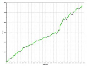
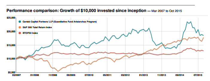
The overall performance of the strategy is quite good.  Average monthly PNL over the period from April to Oct 2015 is almost $8,000 per contract, after fees, with a standard deviation of only $5,500. That equates to an annual Sharpe Ratio in the region of 5.0.  On a decent execution platform the strategy should scale to around 10-15 contracts, with an annual PNL of around $1.0 to $1.5 million.

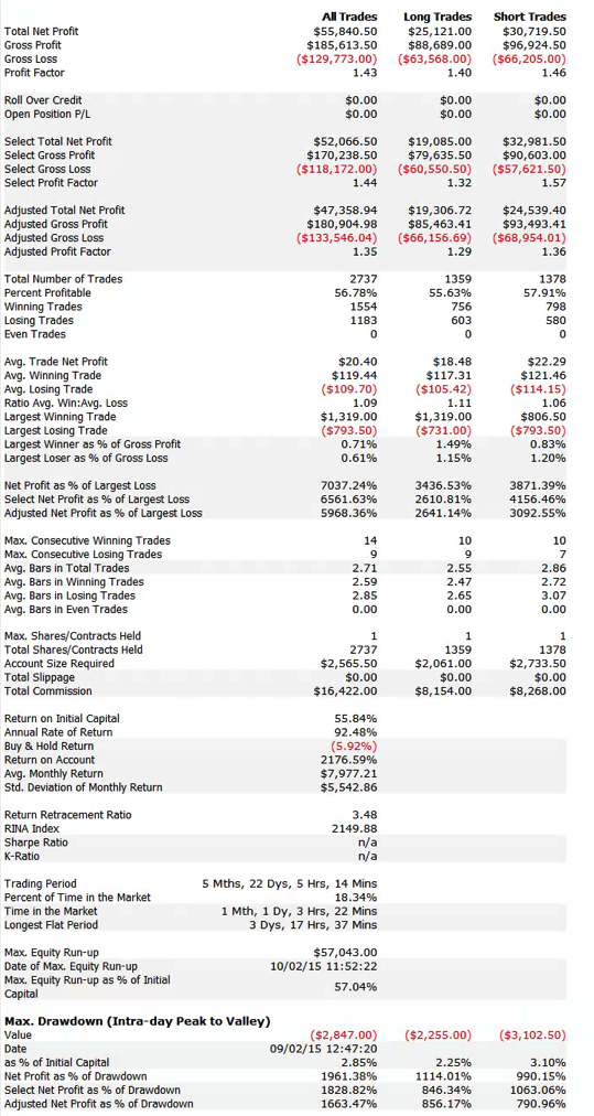
Looking into the performance more closely we find that the win rate (56%) and profit factor (1.43) are typical for a profitable strategy of medium frequency, trading around 20 times per session (in this case from 9:30AM to 4PM EST).

fig2

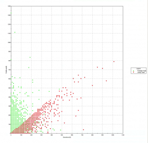
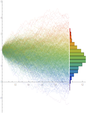
Another attractive feature of the strategy risk profile is the Max Adverse Execution, the drawdown experienced in individual trades (rather than the realized drawdown). In the chart below we see that the MAE increases steadily, without major outliers, to a maximum of only around $1,000 per contract.

Fig3

One concern is that the average trade PL is rather small – $20, just over 1.5 ticks. Strategies that enter and exit with limit orders and have small average trade are generally highly dependent on the fill rate – i.e. the proportion of limit orders that are filled.  If the fill rate is too low, the strategy will be left with too many missed trades on entry or exit, or both.  This is likely to damage strategy performance, perhaps to a significant degree – see, for example my post on High Frequency Trading Strategies.

The fill rate is dependent on the number of limit orders posted at the extreme high or low of the bar, known as the extreme hit rate.  In this case the strategy has been designed specifically to operate at an extreme hit rate of only around 10%, which means that, on average, only around one trade in ten occurs at the high or low of the bar.  Consequently, the strategy is not highly fill-rate dependent and should execute satisfactorily even on a retail platform like Tradestation or Interactive Brokers.

Drivers of Strategy Performance

So far so good.  But before we put the strategy into production, let’s try to understand some of the key factors that determine its performance.  Hopefully that way we will be better placed to judge how profitable the strategy is likely to be as market conditions evolve.

In fact, we have already identified one potential key performance driver: the extreme hit rate (required fill rate) and determined that it is not a major concern in this case. However, in cases where the extreme hit rate rises to perhaps 20%, or more, the fill ratio is likely to become a major factor in determining the success of the strategy.  It would be highly inadvisable to attempt implementation of such a strategy on a retail platform.

SSALGOTRADING AD

What other factors might affect strategy performance?  The correct approach here is to apply the scientific method:  develop some theories about the drivers of performance and see if we can find evidence to support them.

For this case study we might conjecture that, since the strategy enters and exits using limit orders, it should exhibit characteristics of a mean reversion strategy, which will tend to do better when the market moves sideways and rather worse in a strongly trending market.

Another hypothesis is that, in common with most day-trading and high frequency strategies, this strategy will produce better results during periods of higher market volatility.  Empirically, HFT firms have always produced higher profits during volatile market conditions  – 2008 was a banner year for many of them, for example.  In broad terms, times when the market is whipsawing around create additional opportunities for strategies that seek to exploit temporary mis-pricings.  We shall attempt to qualify this general understanding shortly.  For now let’s try to gather some evidence that might support the hypotheses we have formulated.

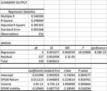
I am going to take a very simple approach to this, using linear regression analysis.  It’s possible to do much more sophisticated analysis using nonlinear methods, including machine learning techniques. In our regression model the dependent variable will be the daily strategy returns.  In the first iteration, let’s use measures of market returns, trading volume and market volatility as the independent variables.

Fig4

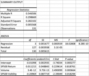
The first surprise is the size of the (adjusted) R Square – at 28%, this far exceeds the typical 5% to 10% level achieved in most such regression models, when applied to trading systems.  In other words, this model does a very good job of account for a large proportion of the variation in strategy returns.

Note that the returns in the underlying S&P50o index play no part (the coefficient is not statistically significant). We might expect this: ours is is a trading strategy that is not specifically designed to be directional and has approximately equivalent performance characteristics on both the long and short side, as you can see from the performance report.

Now for the next surprise: the sign of the volatility coefficient.  Our ex-ante hypothesis is that the strategy would benefit from higher levels of market volatility.  In fact, the reverse appears to be true (due to the  negative coefficient).  How can this be?  On further reflection, the reason why most HFT strategies tend to benefit from higher market volatility is that they are momentum strategies.  A momentum strategy typically enters and exits using market orders and hence requires  a major market move to overcome the drag of the bid-offer spread (assuming it calls the market direction correctly!).  This strategy, by contrast, is a mean-reversion strategy, since entry/exits are effected using limit orders.  The strategy wants the S&P500 index to revert to the mean – a large move that continues in the same direction is going to hurt, not help, this strategy.

Note, by contrast, that the coefficient for the volume factor is positive and statistically significant.  Again this makes sense:  as anyone who has traded the e-mini futures overnight can tell you, the market tends to make major moves when volume is light – simply because it is easier to push around.  Conversely, during a heavy trading day there is likely to be significant opposition to a move in any direction.  In other words, the market is more likely to trade sideways on days when trading volume is high, and this is beneficial for our strategy.

The final surprise and perhaps the greatest of all, is that the strategy alpha appears to be negative (and statistically significant)!  How can this be?  What the regression analysis  appears to be telling us is that the strategy’s performance is largely determined by two underlying factors, volume and volatility.

Let’s dig into this a little more deeply with another regression, this time relating the current day’s strategy return to the prior day’s volume, volatility and market return.

Fig5

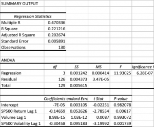
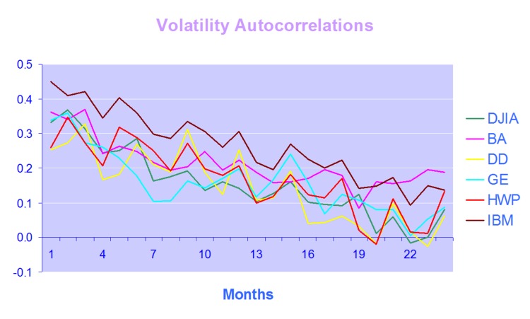
In this regression model the strategy alpha is effectively zero and statistically insignificant, as is the case for lagged volume.  The strategy returns relate inversely to the prior day’s market return, which again appears to make sense for a mean reversion strategy:  our model anticipates that, in the mean, the market will reverse the prior day’s gain or loss.  The coefficient for the lagged volatility factor is once again negative and statistically significant.  This, too, makes sense:  volatility tends to be highly autocorrelated, so if the strategy performance is dependent on market volatility during the current session, it is likely to show dependency on volatility in the prior day’s session also.

So, in summary, we can provisionally conclude that:

This strategy has no market directional predictive power: rather it is a pure, mean-reversal strategy that looks to make money by betting on a reversal in the prior session’s market direction.  It will do better during periods when trading volume is high, and when market volatility is low.

Conclusion

Now that we have some understanding of where the strategy performance comes from, where do we go from here?  The next steps might include some, or all, of the following:

(i) A more sophisticated econometric model bringing in additional lags of the explanatory variables and allowing for interaction effects between them.

(ii) Introducing additional exogenous variables that may have predictive power. Depending on the nature of the strategy, likely candidates might include related equity indices and futures contracts.

(iii) Constructing a predictive model and meta-strategy that would enable us assess the likely future performance of the strategy, and which could then be used to determine position size.  Machine learning techniques can often be helpful in this content.

I will give an example of the latter approach in my next post.

The Lazarus Effect

A perennial favorite with investors, presumably because they are easy to understand and implement, are trades based on a regularly occurring pattern, preferably one that is seasonal in nature.  A well-known example is the Christmas effect, wherein equities generally make their highest risk-adjusted returns during the month of December (and equity indices make the greater proportion of their annual gains in the period from November to January).

As we approach the Easter holiday I thought I might join in the fun with a trade of my own.  There being not much new under the sun, I can assume that there is some ancient trader’s almanac that documents the effect I am about to describe.  If so, I apologize in advance if this is duplicative.

The Pattern of Returns in the S&P 500 Index Around Easter

I want to look at the pattern of pre- and post- Easter returns in the S&P 500 index using weekly data from 1950  (readers can of course substitute the index, ETF or other tradable security in a similar analysis).

The first question is whether there are significant differences (economic and statistical) in index returns in the weeks before and after Easter, compared to a regular week.

Fig 1

It is perhaps not immediately apparent from the smooth histogram plot above, but a whisker plot gives a clearer indication of the disparity in the distributions of returns in the post-Easter week vs. regular weeks.

Fig 2

It is evident that chief distinction is not in the means of the distributions, but in their variances.

A t-test (with unequal variances) confirms that the difference in average returns in the index in the post-Easter week vs. normal weeks is not statistically significant.

Fig 3 It appears that there is nothing special about Index returns in the post-Easter period.

SSALGOTRADING AD

The Lazarus Effect

Hold on – not so fast.  Suppose we look at conditional returns: that is to say, we consider returns in the post-Easter week for holiday periods in which the index sold off in the  week prior to Easter.

There are 26 such periods in the 65 years since 1950 and when we compare the conditional distribution of index returns for these periods against the unconditional distribution of weekly returns we appear to find significant differences in the distributions.  Not only is the variance of the conditional returns much tighter, the mean is clearly higher than the unconditional weekly returns.

Fig 6


Fig 5


The comparison is perhaps best summarized in the following table.  Here we can see that the average conditional return is more than twice that of the unconditional return in the post-Easter week and almost 4x as large as the average weekly return in the index.  The standard deviation in conditional returns for the post-Easter week is less than half that of the unconditional weekly return, producing and information ratio that is almost 10x larger.  Furthermore, of the 26 periods in which the index return in the week prior to Easter was negative, 22 (85%) produced a positive return in the week after Easter (compared to a win rate of only 57% for unconditional weekly returns.

Fig 4

A t-test of conditional vs. unconditional weekly returns confirms that the 58bp difference in conditional vs unconditional (all weeks) average returns is statistically significant at the 0.2% level.

Fig 7

Our initial conclusion, therefore, is that there appears to be a statistically significant pattern in the conditional returns in the S&P 500 index around the post-Easter week. Specifically, the returns in the post-Easter week tend to be much higher than average for  periods in which the pre-Easter weekly returns were negative.

More simply, the S&P 500 index tends to rebound strongly in the week after Easter – a kind of “Lazarus” effect.

 Lazarus – Or Not?

Hold on – not so fast.   What’s so special about Easter?  Yes, I realize it’s topical.  But isn’t this so-called Lazarus effect just a manifestation of the usual mean-reversion in equity index returns?  There is a tendency for weekly returns in the S&P 500 index to “correct” in the week after a downturn.  Maybe the Lazarus effect isn’t specific to Easter.

To examine this hypothesis we need to compare two sets of conditional weekly returns in the S&P 500 index:

A:  Weeks in which the prior week’s return was negative

B:  the subset of A which contains only post-Easter weeks

 If the difference in average returns for sets A and B is not statistically significant, we would conclude that the so-called Lazarus effect is just a manifestation of the commonplace mean reversion in weekly returns.  Only if the average return for the B data set is significant higher than that for set A would we be able to conclude that, in addition to normal mean reversion at weekly frequency, there is an incremental effect specific to the Easter period – the Lazarus effect.

Let’s begin by establishing that there is a statistically significant mean reversion effect in weekly returns in the S&P 500 Index.  Generally, we expect a fall in the index to be followed by a rise (and perhaps vice versa). So we need to  compare the returns in the index for weeks in which the preceding week’s return was positive, vs weeks in which the preceding week’s return was negative.  The t-test below shows the outcome.

Fig 9

The average return in weeks following a downturn is approximately double that during weeks following a rally and the effect is statistically significant at the 3% level.

Given that result, is there any incremental “Lazarus” effect around Easter?  We test that hypothesis by comparing the average returns during the 26 post-Easter weeks which were preceded by a downturn in the index against the average return for all 1,444 weeks which followed a decline in the index.

The t-test shown in the table below confirms that conditional returns in post-Easter weeks are approximately 3x larger on average than returns for all weeks that followed a decline in the index.

Fig 8

Lazarus, it appears, is alive and well.

Happy holidays, all.