An extract from the chapter on pairs trading from my forthcoming book Equity Analytics
Pairs-Trading-1Pairs Trading in the Equities Entity Store


The latest theories, models and investment strategies in quantitative research and trading
An extract from the chapter on pairs trading from my forthcoming book Equity Analytics
Pairs-Trading-1
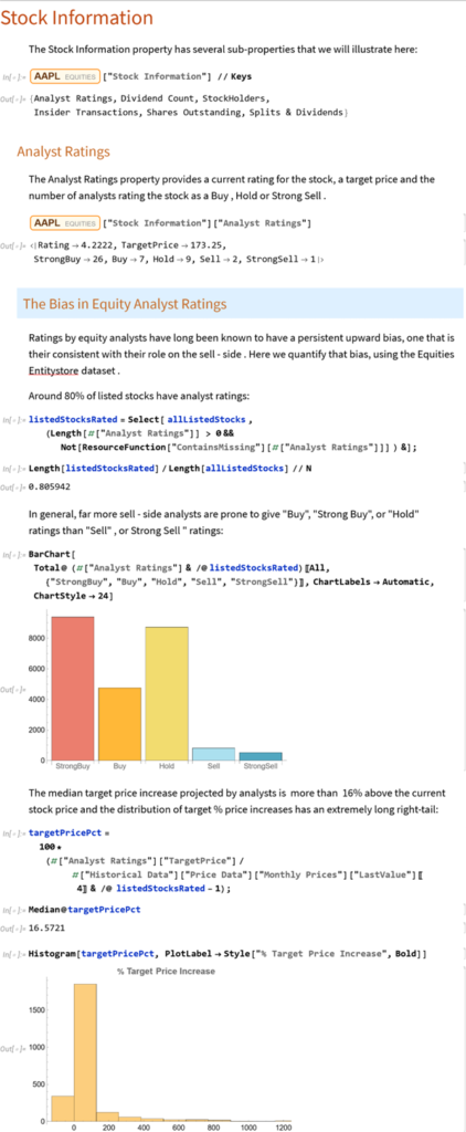
Ratings by equity analysts have long been known to have a persistent upward bias, one that is their consistent with their role on the sell- side. Here we quantify that bias, using the Equities EntityStore dataset.
Full lecture series on Stochastic processes now available on YouTube

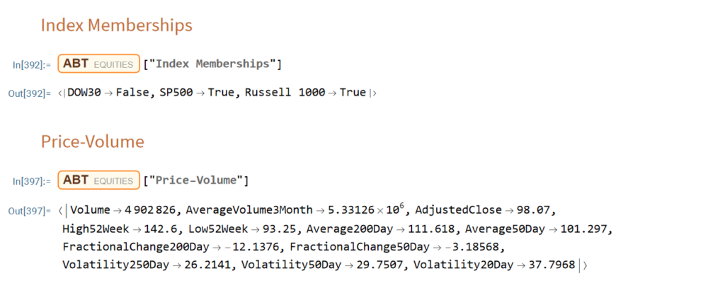
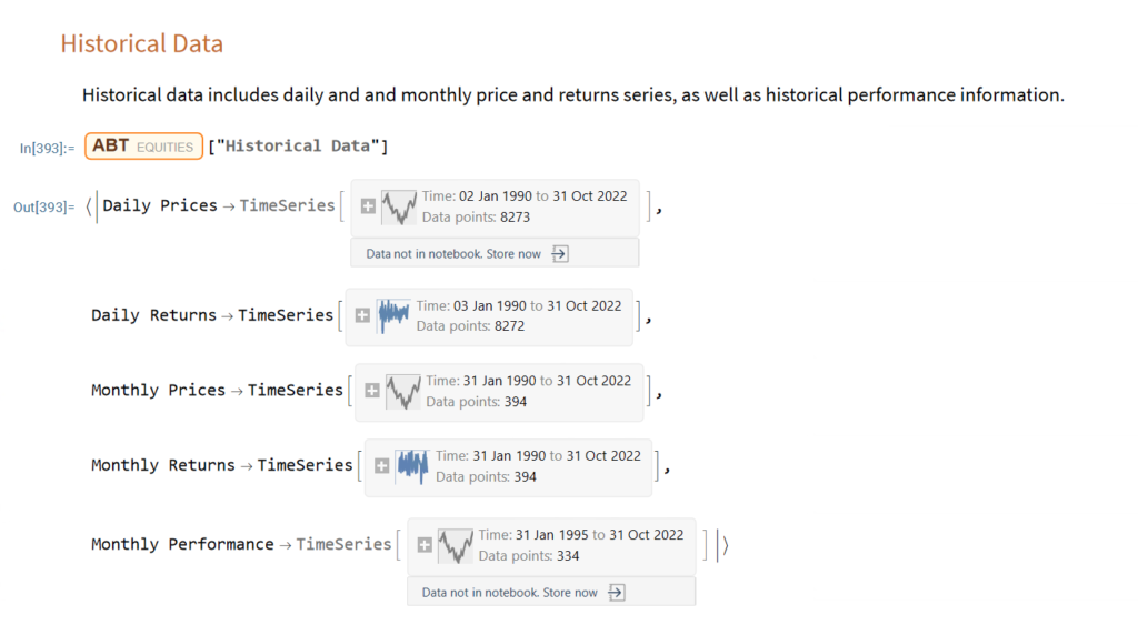
Single Stock Analytics
Generally speaking, one of the major attractions of working in the equities space is that the large number of available securities opens up a much wider range of opportunities for the quantitative researcher than for, say, futures markets. The focus in equities tends to be on portfolio strategies since the scope of the universe permits an unparalleled degree of diversification. Single stock strategies forego such benefit, but they are of interest to the analyst and investor nonetheless: “stock picking” is almost a national pastime, at least for US investors.
Rather than seeking to mitigate stock specific risk through diversification, the stock picker is actively seeking to identify risk opportunities that are unique to a specific stock, and he hopes will yield abnormal returns. These can arise for any number of reasons – mergers and acquisitions, new product development, change in index membership, to name just a few. The hope is that such opportunities may be uncovered by one of several possible means:
One can think of examples of each of these possibilities, but at the same time it has to be admitted that the challenge is very considerable. Firstly, your discovery or methodology would have to be one that has eluded some of the brightest minds in the investment industry. That has happened in the past and will no doubt occur again in future; but the analyst has to have a fairly high regard for his own intellect – or good fortune – to believe that the golden apple will fall into his lap, rather than another’s. Secondly there is the question of the efficient market hypothesis. These days it is fashionable to pour scorn on the EMH, with examples of well-known anomalies often used to justify the opprobrium. But the EMH doesn’t say that markets are 100% efficient, 100% of the time. It says that markets are efficient, on average. This means that there will be times or circumstances in which the market will be efficient and other times and circumstances when it will be relatively inefficient – but you won’t be able to discern which condition the market is in currently. Finally, even if one is successful in identifying such an opportunity, the benefit has to be realizable and economically significant. I can think of several examples of equity strategies that appear to offer the potential to generate alpha, but which turn out to be either unrealizable or economically insignificant after applying transaction costs.
All this is to say that stock picking is one of the most difficult challenges the analyst can undertake. It is also one of the most interesting challenges – and best paid occupations – on Wall Street. So it is unsurprising that for analysts it remains the focus of their research and ambition. In this chapter we will look at some of the ways in which the Equities Entity Store can be used for such purposes and some of the more interesting analytical methods.
Why Technical Analysis Doesn’t Work
Technical Analysis is a very popular approach to analysing stocks. Unfortunately, it is also largely useless, at least if the intention is to uncover potential sources of alpha. The reason is not hard to understand: it relies on applying analytical methods that have been known for decades to widely available public information (price data). There isn’t any source of competitive advantage that might reliably produce abnormal returns. Even the possibility of uncovering a gem amongst the stocks overlooked by other analysts appears increasingly remote these days, as the advent of computerized trading systems has facilitated the application of standard technical analysis tools on an industrial scale. You don’t even need to understand how the indicators work – much less how to program them – in order to apply them to tens of thousands of stocks.
And yet Technical Analysis remains very popular. Why so? The answer, I believe, is because it’s easy to do and can often look very pretty. I will go further and admit that some of the indicators that analysts have devised are extraordinarily creative. But they just don’t work. In fact, I can’t think of another field of human industry that engages so many inventive minds in such a fruitless endeavor.
All this has been clear for some time and yet every year legions of newly minted analysts fling themselves into the task of learning how to apply Technical Analysis to everything from cattle futures to cryptocurrencies. Realistically, the chances of my making any kind of impression on this torrent of pointless hyperactivity are close to zero, but I will give it a go.
A Demonstration
Let’ s begin by picking a stock at random, one I haven’ t look at previously :
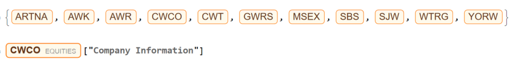
waterUtilities=Select[allListedStocks,#["Sector Information"]["GICS Industry"]== "Water Utilities"&]

We’ll extract a daily price series from 2017 to 2022 and plot an interactive trading chart, to which we can add moving averages, or any number of other technical indicators, as we wish:
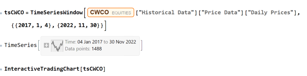
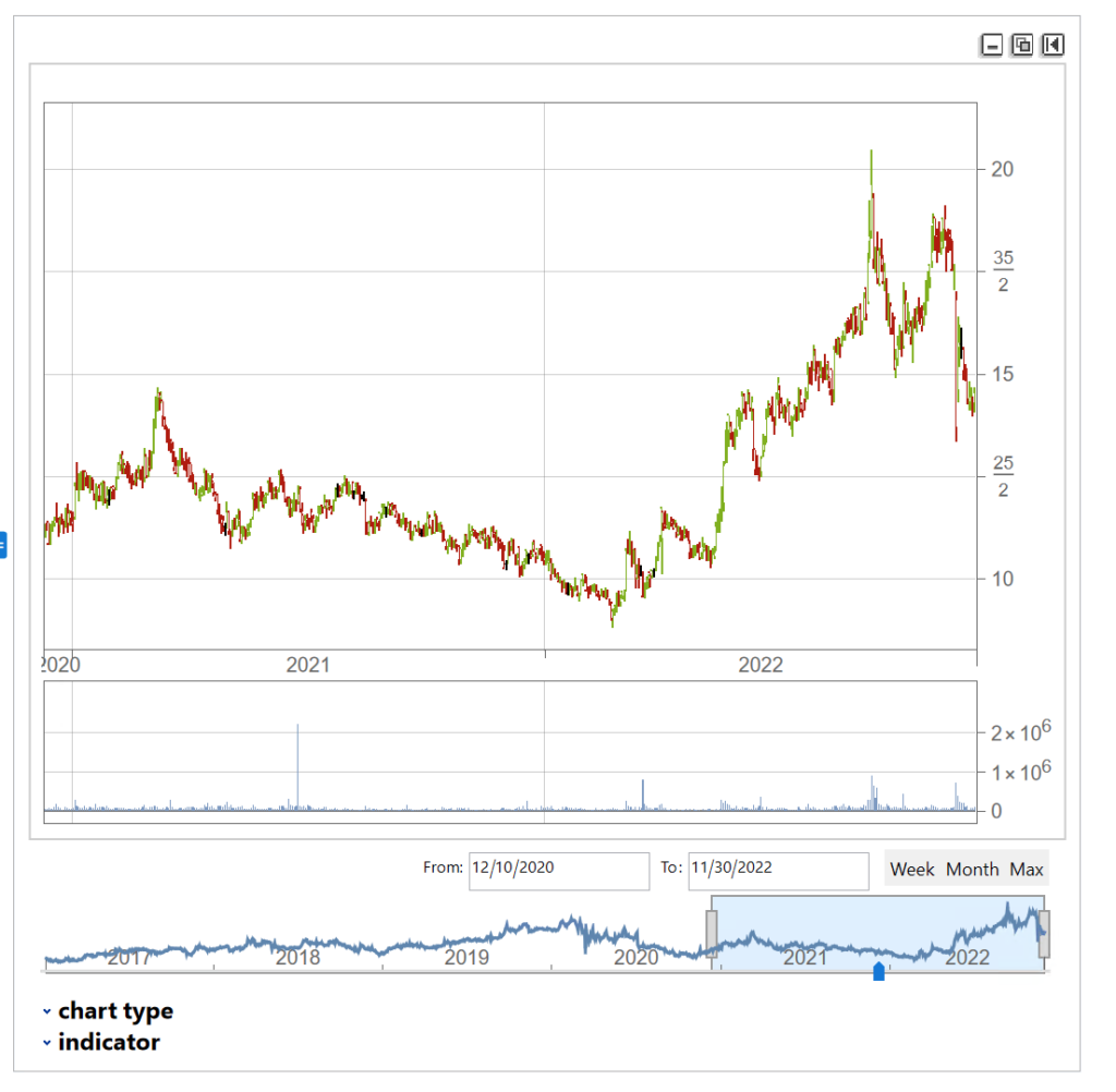
The chart shows several different types of pattern that are well-known to technical analysis, including trends, continuation patterns, gaps, double tops, etc
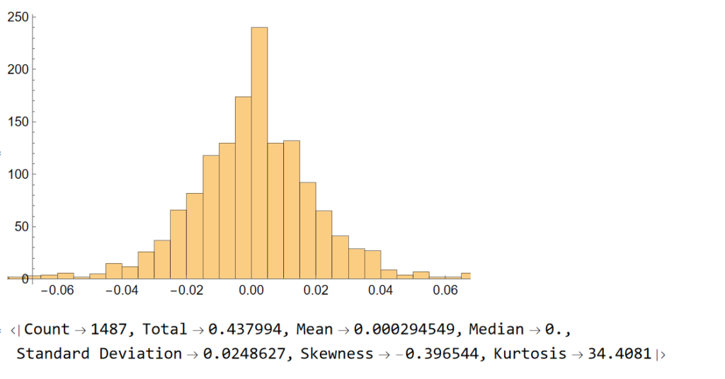
Let’ s look at the pattern of daily returns:
returns=Differences@Log[tsCWCO["PathComponent",4]["Values"]];
Histogram[returns]
stats=ReturnStatistics[returns]
Next, we will generate a series of random returns, drawn from a Gaussian distribution with the same mean and standard deviation as the empirical returns series:
randomreturns=RandomVariate[NormalDistribution[stats["Mean"],stats["Standard Deviation"]],Length[returns]];
Histogram[randomreturns]
ReturnStatistics[randomreturns]
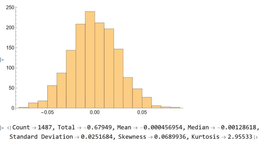
Clearly, the distribution of the generated returns differs from the distribution of empirical returns, but that doesn’t matter: all that counts is that we can agree that the generated returns, which represent the changes in (log) prices from one day to the next, are completely random. Consequently, knowing the random returns, or prices, at time t = 1, 2, . . . , (t-1) in no way enables you to forecast the return , or price, at time t.
Now let’ s generate a series of synthetic prices and time series, using the synthetic returns to calculate the prices for each period:
syntheticPrices=Exp[FoldList[Plus,Log[First[tsCWCO["FirstValues"]][[1;;4]]],Transpose[ConstantArray[returns,4]]]];

tsSynthetic=TimeSeries[ArrayFlatten@{{syntheticPrices,List/@tsCWCO["PathComponent",5]["Values"]}},{tsCWCO["Dates"]}]

InteractiveTradingChart[tsSynthetic]
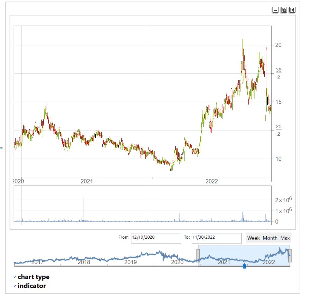
The synthetic time series is very similar to the original and displays many of the same characteristics, including classical patterns that are immediately comprehensible to a technical analyst, such as gaps, reversals , double tops, etc.
But the two time series, although similar, are not identical:
tsCWCO===tsSynthetic

False
We knew this already, of course, because we used randomly generated returns to create the synthetic price series. What this means is that, unlike for the real price series, in the case of the synthetic price series we know for certain that the movement in prices from one period to the next is entirely random. So if prices continue in an upward trend after a gap, or decline after a double top formation appears on the chart of the synthetic series, that happens entirely by random chance, not in response to a pattern flagged by the technical indicator. If we had generated a different set of random returns, we could just as easily have produced a synthetic price series in which prices reversed after a gap up, or continued higher after a double-top formation. Critics of Technical Analysis do not claim that patterns such as gaps, head and shoulders , etc., do not exist – they clearly do. Rather, we say that such patterns are naturally occurring phenomena that will arise even in a series known to be completely random and hence can have no economic significance.
The point is not to say that technical signals never work: sometimes they do and sometimes they don’t. Rather, the point is that, in any given situation, you will be unable to tell whether the signal is going to work this time, or not – because price changes are dominated by random variation.
You can make money in the markets using technical analysis, just as you can by picking stocks at random, throwing darts at a dartboard, or tossing a coin to decide which to buy or sell – i.e. by dumb luck. But you can’t reliably make money this way.

From my forthcoming book Equity Analytics:
Detecting Survivorship Bias
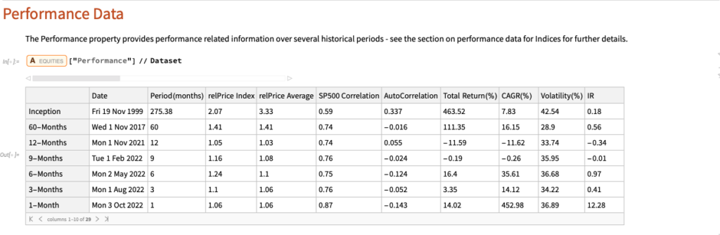
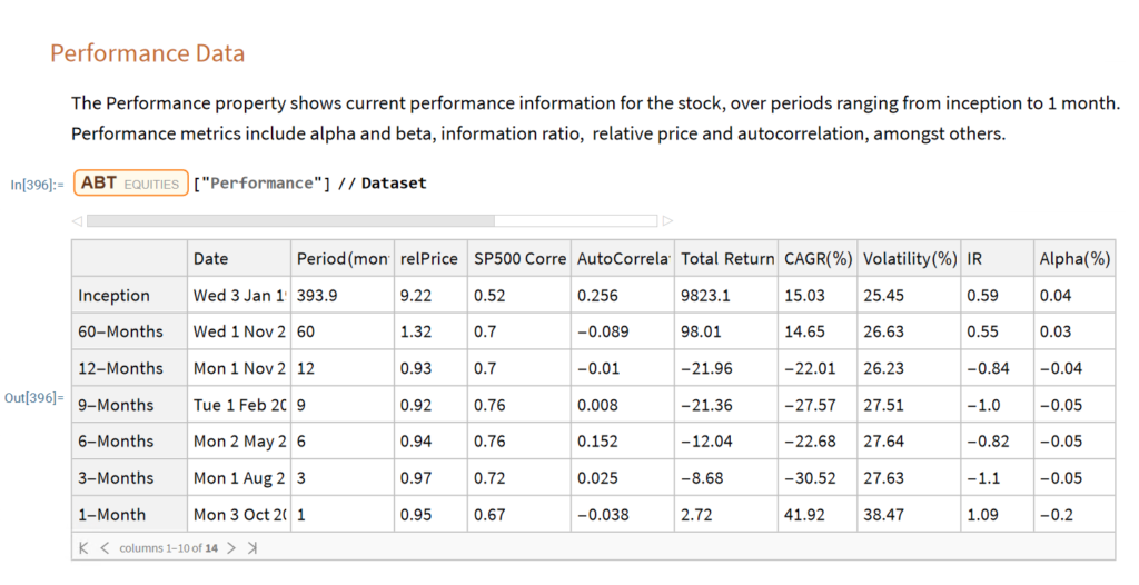
The relprice Index in the Performance Data table shows the price of the stock relative to the S&P 500 index over a specified period.
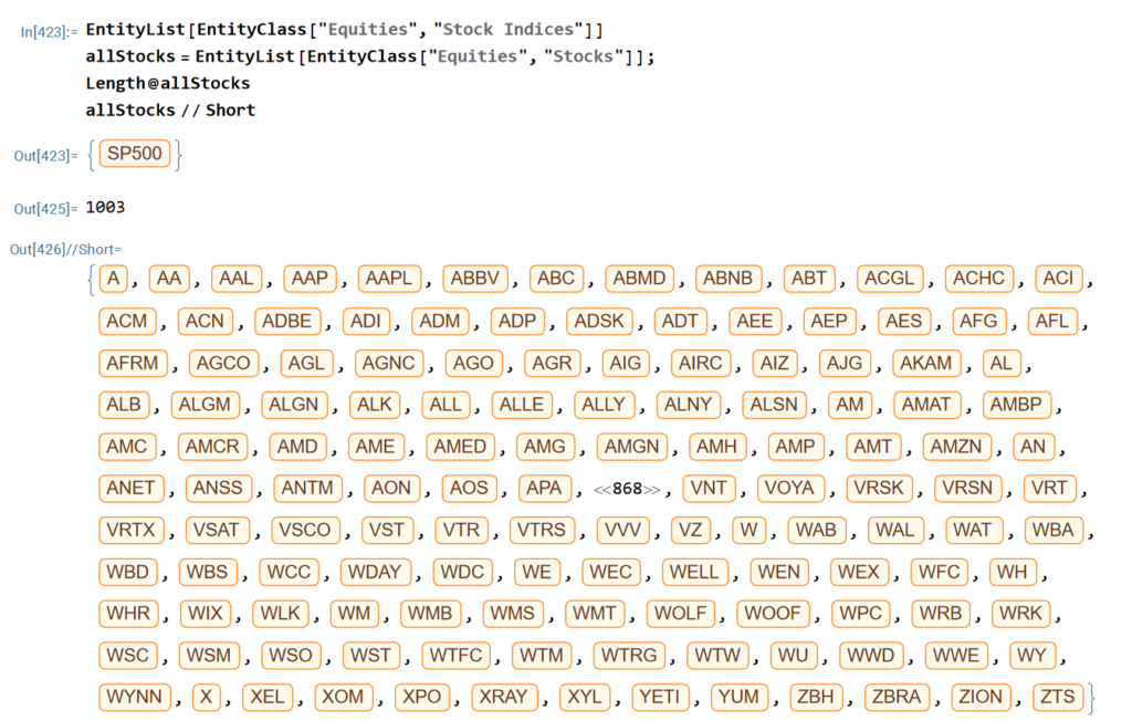
Let’s look at the median relPrice for all stocks that are currently members of the S&P500 index, eliminating any for which the relevant Performance Data is missing:
currentSP500 = Select [ allStocks , # [ Symbol Information ] [ SP500 ] && Length [ # [ Performance ] [ [ All , relPrice Index ] ] ] == 7 & ] // Quiet ;
Sort@RandomSample[currentSP500, 10]

We can then obtain the median relprice for this universe of stocks:
# [ Performance ] [ [ All , relPrice Index ] ] & /@ currentSP500 // Median
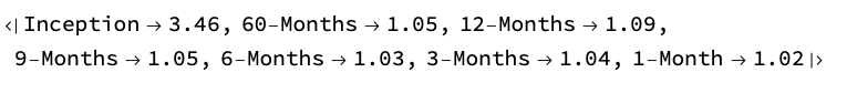
We would expect that roughly half of the S&P 500 index membership would outperform the index over any given period and consequently that the median relPrice would be close to 1. Indeed this is the case for periods of up to 60 months. But if we look at the period from inception, the median relPrice is 3.46 x this level, indicating a very significant out-performance by the current S&P membership relative to the index.
How does this arise? The composition of the index changes over time and many stocks that were once index members have been removed from the index for various reasons. In a small number of cases this will occur where a stock is acquired after a period of exceptional performance. More typically, a stock will be removed from the index after a period of poor performance, following which the firm’s capital structure no longer meets the criteria for inclusion in the index, or because the stock is delisted after acquisition or bankruptcy of the company. None of these stocks is included in the index currently, but instead have been replaced by the stocks of more successful companies – firms that have “survived”. Consequently, when looking the current membership of the index we are considering only these “survivors” and neglecting those stocks that were once index members but which have since been removed. As a result, the aggregate performance of the current members, the survivors, far exceeds the historical performance of the index, which reflects the impact of those stocks removed from membership, mostly for reasons of under-performance.
The outcome of this is that if you design equity portfolio strategies using a universe comprising only the current index membership, or indeed only stocks that are currently listed, the resulting portfolio is subject to this kind of “survivorship bias”, that will tend to inflate its performance. This probably wont make much difference over shorter periods of up to five years, but if you backtest the strategy over longer periods the results are likely to become subject to significant upward bias that will over-state the expected performance of the strategy in future. You may find evidence of this bias in the form of deteriorating strategy performance over time, for more recent periods covered in the backtest.
A secondary effect of using a survivorship-biased universe, also very important, is that it will prove difficult to identify enough short candidates to be able to design long/short or market-neutral strategies. The long term performance of even the worst performing survivors is such that shorting them will almost always detract from portfolio performance without reducing portfolio risk, due to the highly correlated performance amongst survivors. In order to design such strategies, it is essential that your universe contains stocks that are no longer listed, as many of these will have been delisted for reasons of underperformance. These are the ideal short candidates for your long/short or market-neutral strategy.
In summary, it is vital that the stock universe includes both currently listed and delisted stocks in order to mitigate the impact of survivorship bias.
Let’s take a look at the median relPrice once again, this time including both listed and delisted stocks:
allValidStocks = Select [ allStocks , Length [ # [ Performance ] [ [ All , relPrice Index ] ] ] == 7 & ] // Quiet ;
# [ Performance ] [ [ All , relPrice Index ] ] & /@ allValidStocks // Median


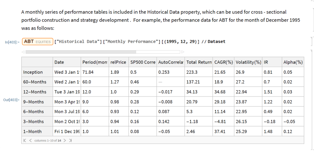
Equities Entity Store – A Brief Review
The Equities Entity Store applies the object-oriented concept of Entity Stores in the Wolfram Language to create a collection of equity objects, both stocks and stock indices, containing current and historical fundamental, technical and performance-related data. Also included in the release version of the product will be a collection of utility functions (a.k.a. “Methods”) that will facilitate equity analysis, the formation and evaluation of equity portfolios and the development and back-testing of equities strategies, including cross-sectional strategies.
In the pre-release version of the store there are just over 1,000 equities, but this will rise to over 2,000 in the first release, as delisted securities are added to the store. This is important in order to eliminate survivor bias from the data set.
First Release of the Equities Entity Store – January 2023
The first release of the equities entity store product will contain around 2,000-2,500 equities, including at least 1,000 active stocks listed on the NYSE and NASDAQ exchanges and a further 1,000-1,500 delisted securities. All of the above information will be available for each equity and, in addition, the historical data will include quarterly fundamental data.
The other major component of the store will be analytics tools, including single-stock analytics functions such as those illustrated here. More important, however, is that the store will contain advanced analytics tools designed to assist the analyst in the construction of optimized equity portfolios and in the development and backtesting of long and long/short equity strategies.
Readers wishing to receive more information should contact me at algosciences (at) gmail.com
Quality Research vs. Poor Research
The stem paper for this post is:
Bao W, Yue J, Rao Y (2017) A deep learning framework for financial time series using
stacked autoencoders and long-short term memory. PLoS ONE 12(7): e0180944. https://doi.org/10.1371/journal.pone.0180944
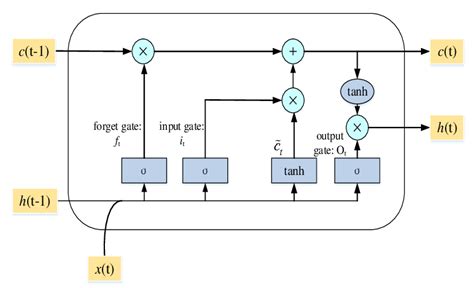
The chief claim by the researchers is that 90% to 95% 1-day ahead forecast accuracy can be achieved for a selection of market indices, including the S&P500 and Dow Jones Industrial Average, using a deep learning network of stacked autoencoders and LSTM layers, acting on data transformed using the Haar Discrete Wavelet Transform. The raw data comprises daily data for the index, around a dozen standard technical indicators, the US dollar index and an interest rate series.
Before we go into any detail let’s just step back and look at the larger picture. We have:
There’s enough red flags here to start a stampede at Pamplona. Let’s go through them one by one:
These simple considerations should be enough for any experienced quant to give the paper a wide berth.
Digging into the Methodology
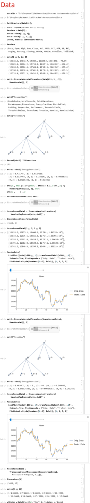
So we start from a raw dataset with variables that closely match those described in the paper (see headers for details). Of course, I don’t know the parameter values they used for most of the technical indicators, but it possibly doesn’t matter all that much.
Note that I am applying DWT using the Haar wavelet twice: once to the original data and then again to the transformed data. This has the effect of filtering out higher frequency “noise” in the data, which is the object of the exercise. If follow this you will also see that the DWT actually adds noisy fluctuations to the US Dollar index and 13-Week TBill series. So these should be excluded from the de-noising process. You can see how the DWT denoising process removes some of the higher frequency fluctuations from the opening price, for instance:
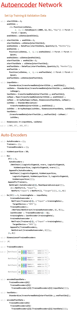
2. Stacked Autoencoders
First up, we need to produce data for training, validation and testing. I am doing this for just the first batch of data. We would then move the window forward + 3 months, rinse and repeat.
Note that:
(1) The data is being standardized. If you don’t do this the outputs from the autoencoders is mostly just 1s and 0s. Same happens if you use Min/Max scaling.
(2) We use the mean and standard deviation from the training dataset to normalize the test dataset. This is a trap that too many researchers fall into – standardizing the test dataset using the mean and standard deviation of the test dataset is feeding forward information.
The Autoencoder stack uses a hidden layer of size 10 in each encoder. We strip the output layer from the first encoder and use the hidden layer as inputs to the second autoencoder, and so on:
3. Benchmark Model
Before we plow on any further lets do a sanity check. We’ll use the Predict function to see if we’re able to get any promising-looking results. Here we are building a Gradient Boosted Trees predictor that maps the autoencoded training data to the corresponding closing prices of the index, one step ahead.
Next we use the predictor on the test dataset to produce 1-step-ahead forecasts for the closing price of the index.
Finally, we construct a trading model, as described in the paper, in which we go long or short the index depending on whether the forecast is above or below the current index level. The results do not look good (see below).
Now, admittedly, an argument can be made that a properly constructed LSTM model would outperform a simple gradient-boosted tree – but not by the amount that would be required to improve the prediction accuracy from around 50% to nearer 95%, the level claimed in the paper. At most I would expect to see a 1% to 5% improvement in forecast accuracy.
So what this suggests to me is that the researchers have got something wrong, by somehow allowing forward information to leak into the modeling process. The most likely culprits are:
A More Complete Attempt to Replicate the Research
There’s a much more complete attempt at replicating the research in this Git repo
As the repo author writes:
My attempts haven’t been succesful so far. Given the very limited comments regarding implementation in the article, it may be the case that I am missing something important, however the results seem too good to be true, so my assumption is that the authors have a bug in their own implementation. I would of course be happy to be proven wrong about this statement 😉
Conclusion
Over time, as one’s experience as a quant deepens, you learn to recognize the signs of shoddy research and save yourself the effort of trying to replicate it. It’s actually easier these days for researchers to fool themselves (and their readers) that they have uncovered something interesting, because of the facility with which complex algorithms can be deployed in an inappropriate way.
Postscript
This paper echos my concerns about the incorrect use of wavelets in a forecasting context:
The incorrect development of these wavelet-based forecasting models occurs during wavelet decomposition (the process of extracting high- and low-frequency information into different sub-time series known as wavelet and scaling coefficients, respectively) and as a result introduces error into the forecast model inputs. The source of this error is due to the boundary condition that is associated with wavelet decomposition (and the wavelet and scaling coefficients) and is linked to three main issues: 1) using ‘future data’ (i.e., data from the future that is not available); 2) inappropriately selecting decomposition levels and wavelet filters; and 3) not carefully partitioning calibration and validation data.


In my last post I mapped out how one could test the reliability of a single stock strategy (for the S&P 500 Index) using synthetic data generated by the new algorithm I developed.
As this piece of research follows a similar path, I won’t repeat all those details here. The key point addressed in this post is that not only are we able to generate consistent open/high/low/close prices for individual stocks, we can do so in a way that preserves the correlations between related securities. In other words, the algorithm not only replicates the time series properties of individual stocks, but also the cross-sectional relationships between them. This has important applications for the development of portfolio strategies and portfolio risk management.
KO-PEP Pair
To illustrate this I will use synthetic daily data to develop a pairs trading strategy for the KO-PEP pair.
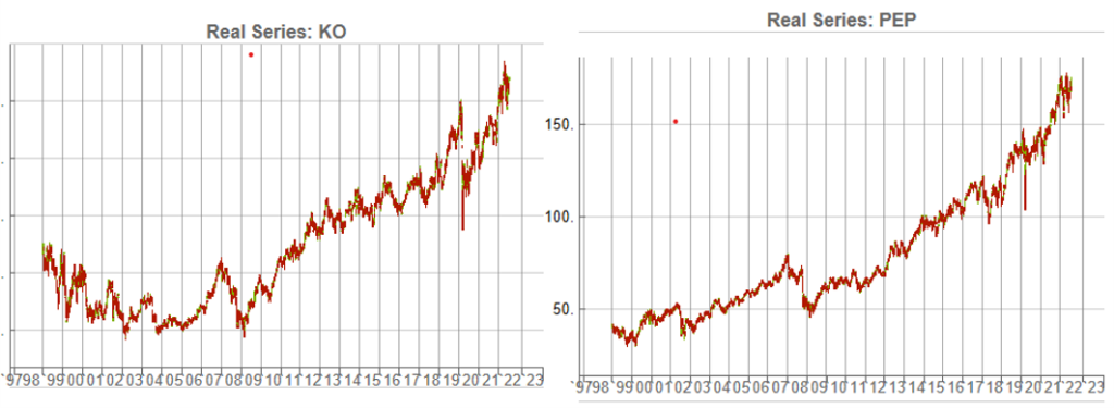
The two price series are highly correlated, which potentially makes them a suitable candidate for a pairs trading strategy.
There are numerous ways to trade a pairs spread such as dollar neutral or beta neutral, but in this example I am simply going to look at trading the price difference. This is not a true market neutral approach, nor is the price difference reliably stationary. However, it will serve the purpose of illustrating the methodology.
Obviously it is crucial that the synthetic series we create behave in a way that replicates the relationship between the two stocks, so that we can use it for strategy development and testing. Ideally we would like to see high correlations between the synthetic and original price series as well as between the pairs of synthetic price data.
We begin by using the algorithm to generate 100 synthetic daily price series for KO and PEP and examine their properties.
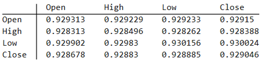
Correlations
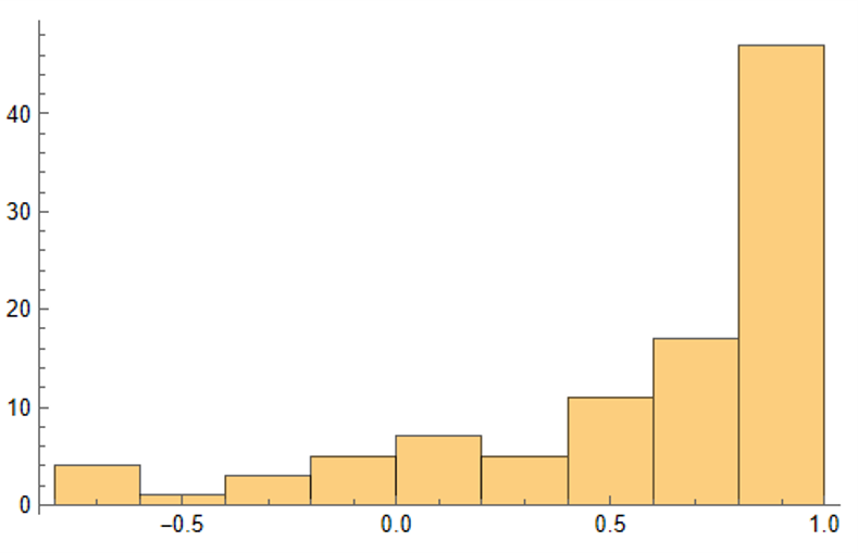
As we saw previously, the algorithm is able to generate synthetic data with correlations to the real price series ranging from below zero to close to 1.0:
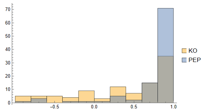
The crucial point, however, is that the algorithm has been designed to also preserve the cross-sectional correlation between the pairs of synthetic KO-PEP data, just as in the real data series:
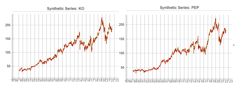
Some examples of highly correlated pairs of synthetic data are shown in the plots below:
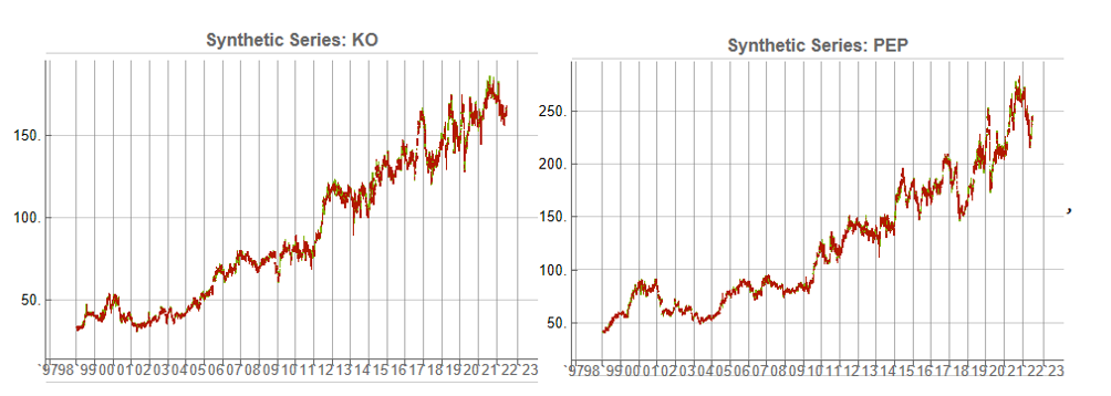
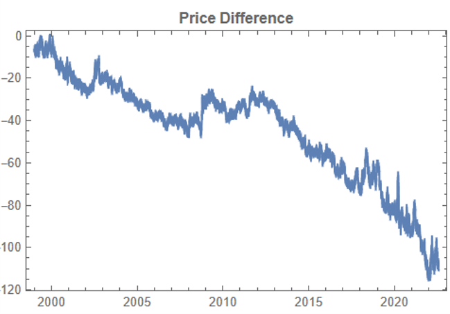
In addition to correlation, we might also want to consider the price differences between the pairs of synthetic series, since the strategy will be trading that price difference, in the simple approach adopted here. We could, for example, select synthetic pairs for which the divergence in the price difference does not become too large, on the assumption that the series difference is stationary. While that approach might well be reasonable in other situations, here an assumption of stationarity would be perhaps closer to wishful thinking than reality. Instead we can use of selection of synthetic pairs with high levels of cross-correlation, as we all high levels of correlation with the real price data. We can also select for high correlation between the price differences for the real and synthetic price series.
Strategy Development & WFO Testing
Once again we follow the procedure for strategy development outline in the previous post, except that, in addition to a selection of synthetic price difference series we also include 14-day correlations between the pairs. We use synthetic daily synthetic data from 1999 to 2012 to build the strategy and use the data from 2013 onwards for testing/validation. Eventually, after 50 generations we arrive at the result shown in the figure below:
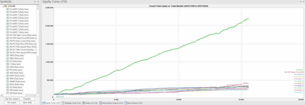
As before, the equity curve for the individual synthetic pairs are shown towards the bottom of the chart, while the aggregate equity curve, which is a composition of the results for all none synthetic pairs is shown above in green. Clearly the results appear encouraging.
As a final step we apply the WFO analysis procedure described in the previous post to test the performance of the strategy on the real data series, using a variable number in-sample and out-of-sample periods of differing size. The results of the WFO cluster test are as follows:
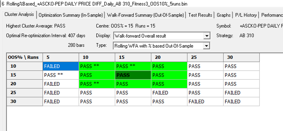
The results are no so unequivocal as for the strategy developed for the S&P 500 index, but would nonethless be regarded as acceptable, since the strategy passes the great majority of the tests (in addition to the tests on synthetic pairs data).
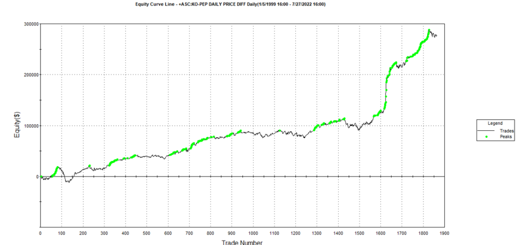
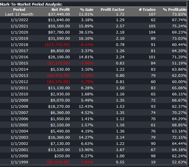
The final results appear as follows:
Conclusion
We have demonstrated how the algorithm can be used to generate synthetic price series the preserve not only the important time series properties, but also the cross-sectional properties between series for correlated securities. This important feature has applications in the development of statistical arbitrage strategies, portfolio construction methodology and in portfolio risk management.