Copulas in Risk Management

QUANTITATIVE RESEARCH AND TRADING
The latest theories, models and investment strategies in quantitative research and trading


Text and sentiment analysis has become a very popular topic in quantitative research over the last decade, with applications ranging from market research and political science, to e-commerce. In this post I am going to outline an approach to the subject, together with some core techniques, that have applications in investment strategy.
In the early days of the developing field of market sentiment analysis, the supply of machine readable content was limited to mainstream providers of financial news such as Reuters or Bloomberg. Over time this has changed with the entry of new competitors in the provision of machine readable news, including, for example, Ravenpack or more recent arrivals like Accern. Providers often seek to sell not only the raw news feed service, but also their own proprietary sentiment indicators that are claimed to provide additional insight into how individual stocks, market sectors, or the overall market are likely to react to news. There is now what appears to be a cottage industry producing white papers seeking to demonstrate the value of these services, often accompanied by some impressive pro-forma performance statistics for the accompanying strategies, which include long-only, long/short, market neutral and statistical arbitrage.
For the purpose of demonstration I intend to forego the blandishments of these services, although many are no doubt are excellent, since the reader is perhaps unlikely to have access to them. Instead, in what follows I will focus on a single news source, albeit a highly regarded one: the Wall Street Journal. This is, of course, a simplification intended for illustrative purposes only – in practice one would need to use a wide variety of news sources and perhaps subscribe to a machine readable news feed service. But similar principles and techniques can be applied to any number of news feeds or online sites.
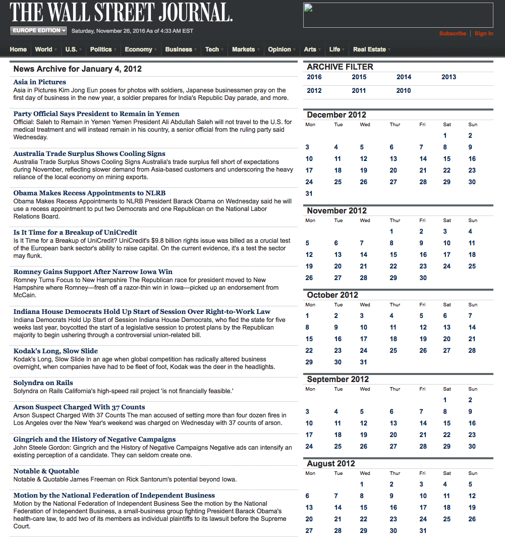
We are going to access the Journal’s online archive, which presents daily news items in a convenient summary format, an example of which is shown below. The archive runs from the beginning of 2012 through to the current day, providing ample data for analysis. In what follows, I am going to make two important assumptions, neither of which is likely to be 100% accurate – but which will not detract too much from the validity of the research, I hope. The first assumption is that the news items shown in each daily archive were reported prior to the market open at 9:30 AM. This is likely to be true for the great majority of the stories, but there are no doubt important exceptions. Since we intend to treat the news content of each archive as antecedent to the market action during the corresponding trading session, exceptions are likely to introduce an element of look-ahead bias. The second assumption is that the archive for each day is shown in the form in which it would have appeared on the day in question. In reality, there are likely to have been revisions to some of the stories made subsequent to their initial publication. So, here too, we must allow for the possibility of look-ahead bias in the ensuing analysis.
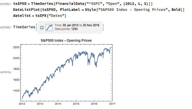
With those caveats out of the way, let’s proceed. We are going to be using broad market data for the S&P 500 index in the analysis to follow, so the first step is to download daily price series for the index. Note that we begin with daily opening prices, since we intend to illustrate the application of news sentiment analysis with a theoretical day-trading strategy that takes positions at the start of each trading session, exiting at market close.
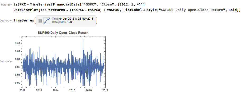
From there we calculate the intraday return in the index, from market open to close, as follows:
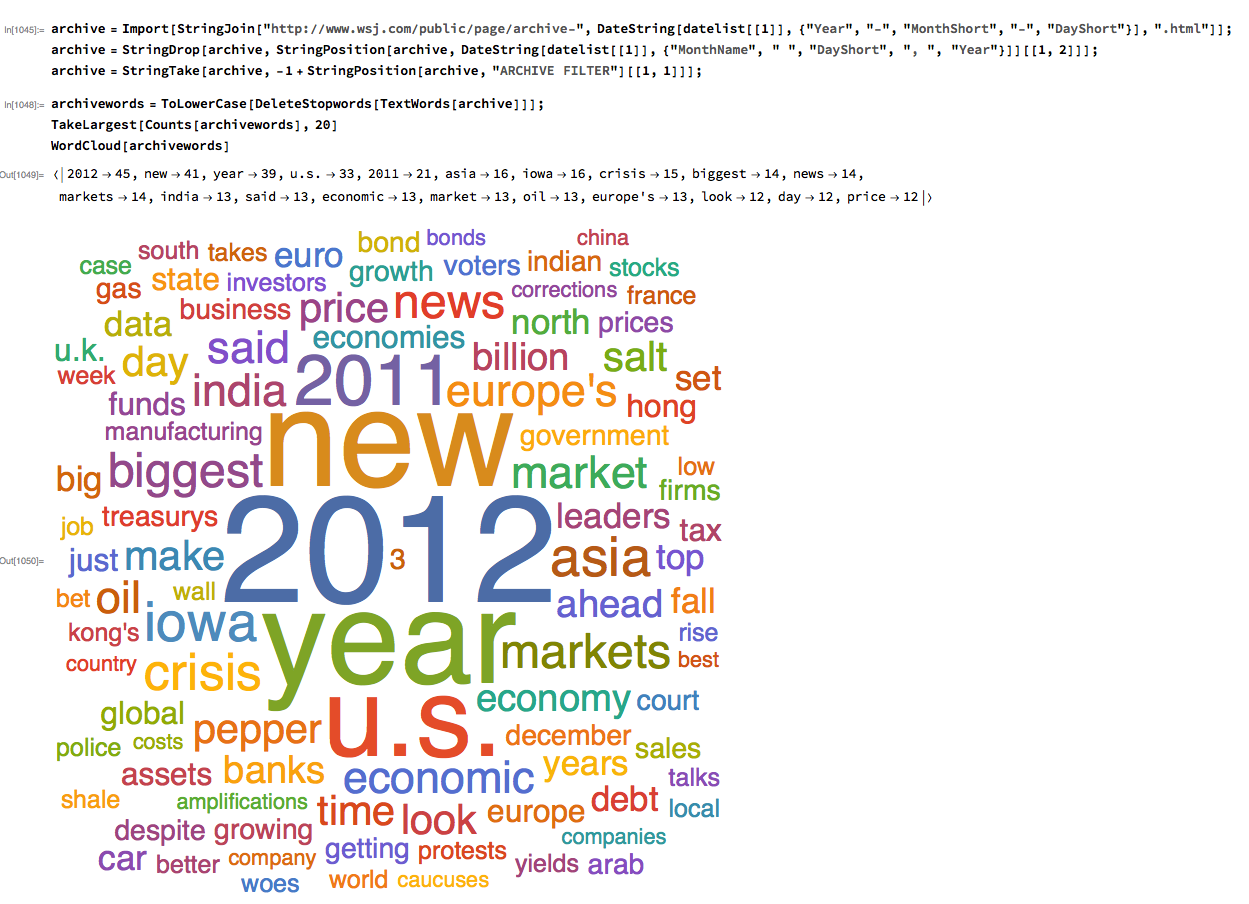
Next we turn to the task of reading the news archive and categorizing its content. Mathematica makes the importation of html pages very straightforward, and we can easily crop the raw text string to exclude page headers and footers. The approach I am going to take is to derive a sentiment indicator based on an analysis of the sentiment of each word in the daily archive. Before we can do that we must first convert the text into individuals words, stripping out standard stop-words such as “the” and “in” and converting all the text to lower case. Naturally one can take this pre-processing a great deal further, by identifying and separating out proper nouns, for example. Once the text processing stage is complete we can quickly summarize the content, for example by looking at the most common words, or by representing the entire archive in the form of a word cloud. Given that we are using the archive for the first business day of 2012, it is perhaps unsurprising that we find that “2012”, “new” and “year” feature so prominently!
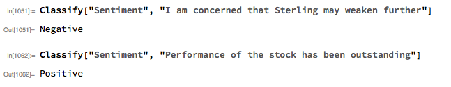
The subject of sentiment analysis is a complex one and I only touch on it here. For those interested in the subject I can recommend The Text Mining Handbook, by Feldman and Sanger, which is a standard work on the topic. Here I am going to employ a machine learning classifier provided with Mathematica 11. It is not terribly sophisticated (or, at least, has not been developed with financial applications especially in mind), but will serve for the purposes of this article. For those unfamiliar with the functionality, the operation of the sentiment classification algorithm is straightforward enough. For instance:
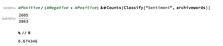
We apply the algorithm to classify each word in the daily news archive and arrive at a sentiment indicator based on the proportion of words that are classified as “positive”. The sentiment reading for the archive for Jan-3, 2012, for example, turns out to be 67.4%:
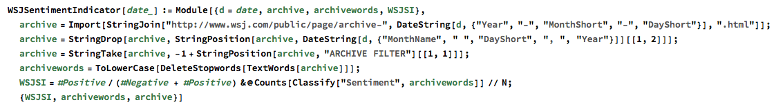
We can automate the process of classifying the entire WSJ archive with just a few lines of code, producing a time series for the daily sentiment indicator, which has an average daily value of 68.5% – the WSJ crowd tends to be bullish, clearly! Note how the 60-day moving average of the indicator rises steadily over the period from 2012 through Q1 2015, then abruptly reverses direction, declining steadily thereafter – even somewhat precipitously towards the end of 2016.

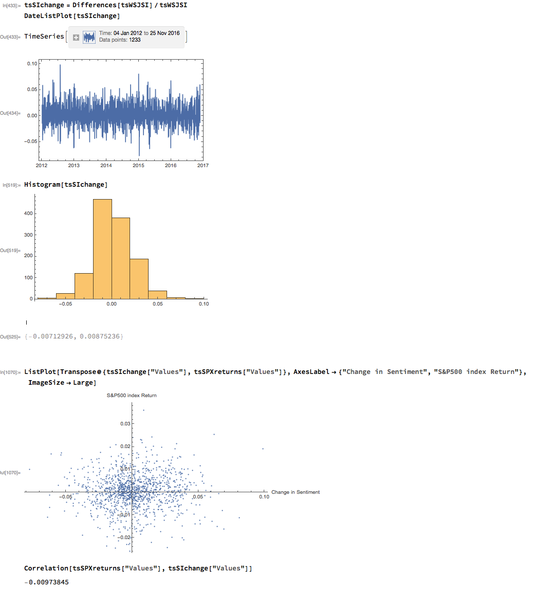
As with most data series in investment research, we are less interested in the level of a variable, such as a stock price, than we are in the changes in level. So the next step is to calculate the daily percentage change in the sentiment indicator and examine the correlation with the corresponding intraday return in the S&P 500 Index. At first glance our sentiment indicator appears to have very little predictive power – the correlation between indicator changes and market returns is negligibly small overall – but we shall later see that this is not the last word.
Thus far the results appear discouraging; but as is often the case with this type of analysis we need to look more closely at the conditional distribution of returns. Specifically, we will examine the conditional distribution of S&P 500 Index returns when changes in the sentiment index are in the upper and lower quantiles of the distribution. This will enable us to isolate the impact of changes in market sentiment at times when the swings in sentiment are strongest. In the analysis below, we begin by examining the upper and lower third of the distribution of changes in sentiment:
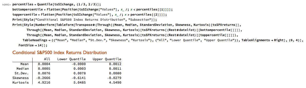
The analysis makes clear that the distribution of S&P 500 Index returns is very different on days when the change in market sentiment is large and positive vs. large and negative. The difference is not just limited to the first moment of the conditional distribution, where the difference in the mean return is large and statistically significant, but also in the third moment. The much larger, negative skewness means that there is a greater likelihood of a large decline in the market on days in which there is a sizable drop in market sentiment, than on days in which sentiment significantly improves. In other words, the influence of market sentiment changes is manifest chiefly through the mean and skewness of the conditional distributions of market returns.
We can capitalize on these effects using a simple trading strategy in which we increase the capital allocated to a long-SPX position on days when market sentiment improves, while reducing exposure on days when market sentiment falls. We increase the allocation by a factor – designated the leverage factor – on days when the change in the sentiment indicator is in the upper 1/3 of the distribution, while reducing the allocation by 1/leveragefactor on days when the change in the sentiment indicator falls in lower 1/3 of the distribution. The allocation on other days is 100%. The analysis runs as follows:

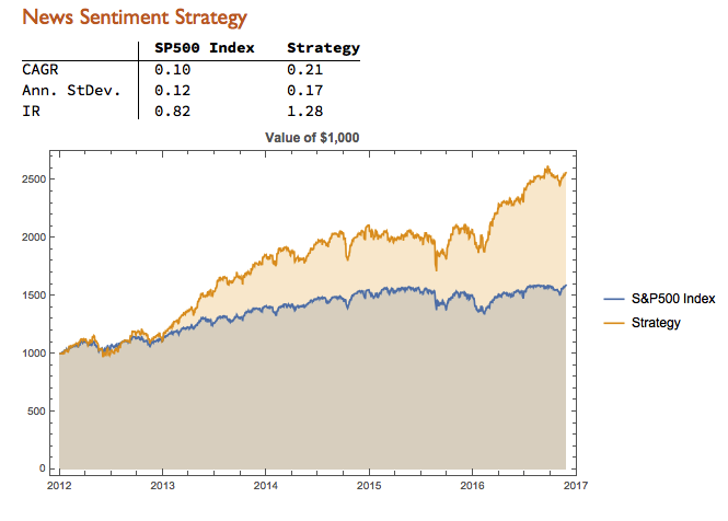
It turns out that, using a leverage factor of 2.0, we can increase the CAGR from 10% to 21% over the period from 2012-2016 using the conditional distribution approach. This performance enhancement comes at a cost, since the annual volatility of the news sentiment strategy is 17% compared to only 12% for the long-only strategy. However, the overall net result is positive, since the risk-adjusted rate of return increases from 0.82 to 1.28.
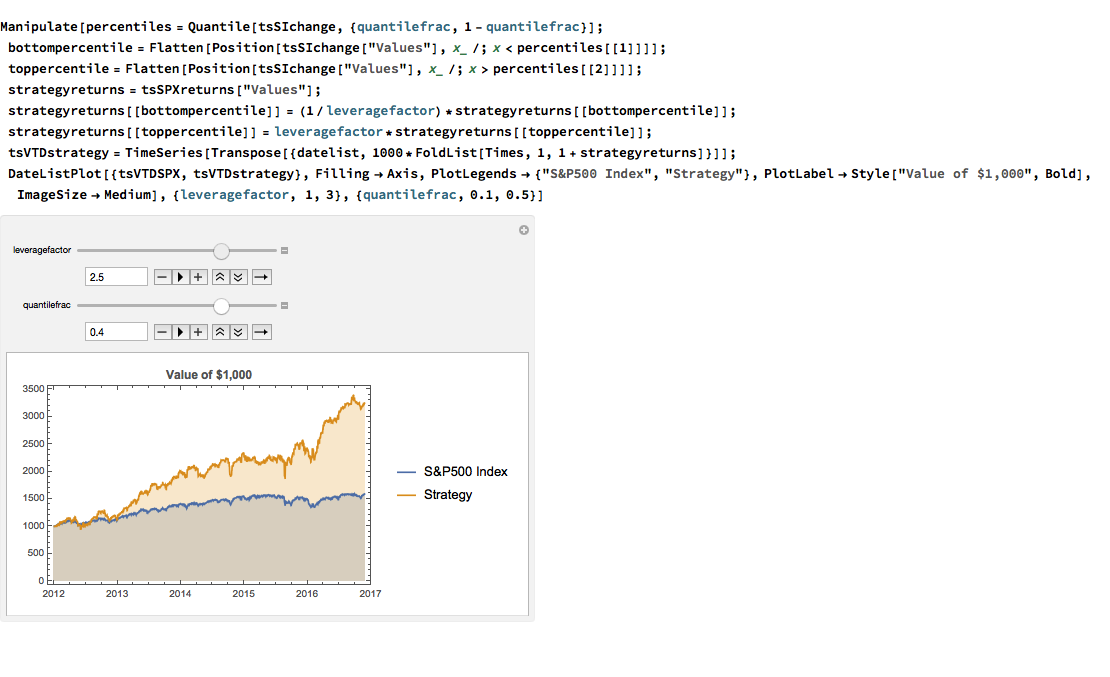
We can explore the robustness of the result, comparing different quantile selections and leverage factors using Mathematica’s interactive Manipulate function:
We have seen that a simple market sentiment indicator can be created quite easily from publicly available news archives, using a standard machine learning sentiment classification algorithm. A market sentiment algorithm constructed using methods as straightforward as this appears to provide the capability to differentiate the conditional distribution of market returns on days when changes in market sentiment are significantly positive or negative. The differences in the higher moments of the conditional distribution appears to be as significant as the differences in the mean. In principle, we can use the insight provided by the sentiment indicator to enhance a long-only day-trading strategy, increasing leverage and allocation on days when changes to market sentiment are positive and reducing them on days when sentiment declines. The performance enhancements resulting from this approach appear to be significant.
Several caveats apply. The S&P 500 index is not tradable, of course, and it is not uncommon to find trading strategies that produce interesting theoretical results. In practice one would be obliged to implement the strategy using a tradable market proxy, such as a broad market ETF or futures contract. The strategy described here, which enters and exits positions daily, would incur substantial trading costs, that would be further exacerbated by the use of leverage.
Of course there are many other uses one can make of news data, in particular with firm-specific news and sentiment analytics, that fall outside the scope of this article. Hopefully, however, the methodology described here will provide a sign-post towards further, more practically useful research.
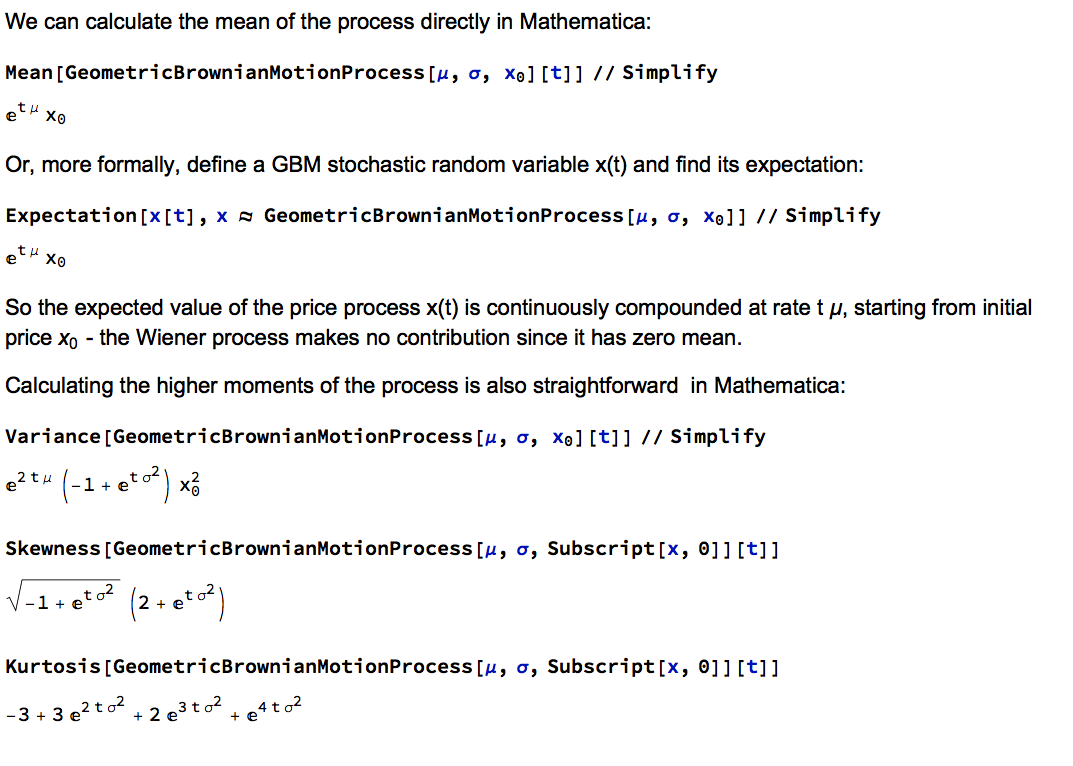
Wolfram Research introduced random processes in version 9 of Mathematica and for the first time users were able to tackle more complex modeling challenges such as those arising in stochastic calculus. The software’s capabilities in this area have grown and matured over the last two versions to a point where it is now feasible to teach stochastic calculus and the fundamentals of financial engineering entirely within the framework of the Wolfram Language. In this post we take a lightening tour of some of the software’s core capabilities and give some examples of how it can be used to create the building blocks required for a complete exposition of the theory behind modern finance.
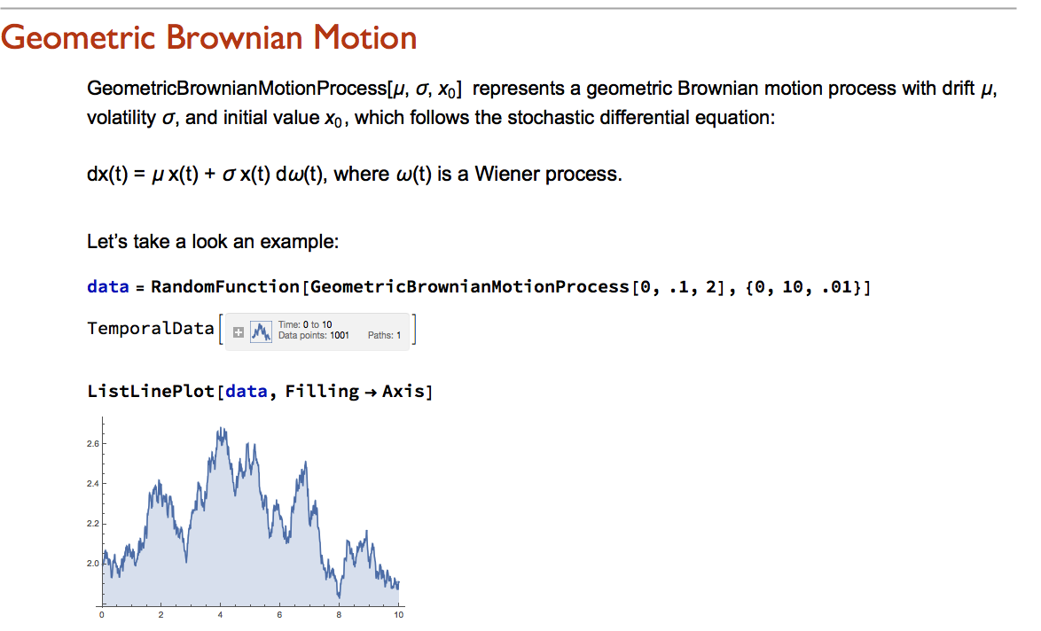
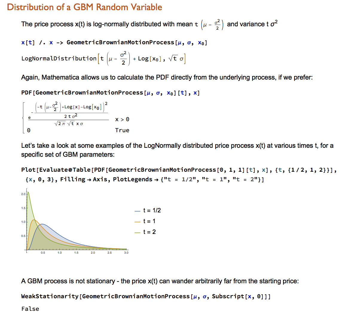
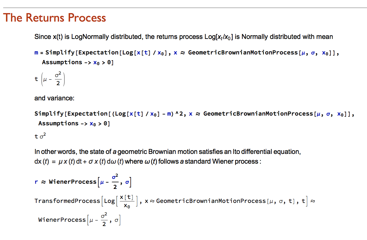


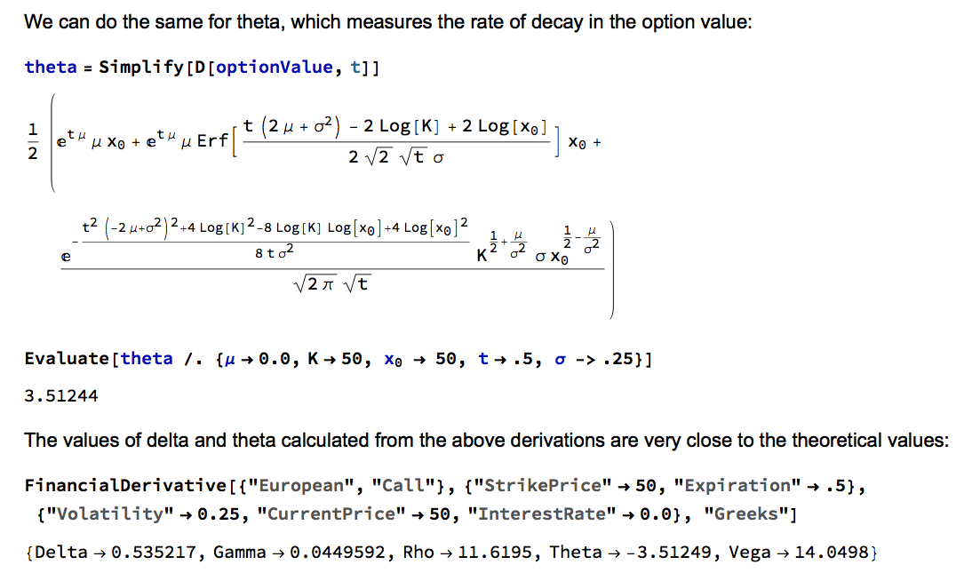
Financial Engineering has long been a staple application of Mathematica, an area in which is capabilities in symbolic logic stand out. But earlier versions of the software lacked the ability to work with Ito calculus and model stochastic processes, leaving the user to fill in the gaps by other means. All that changed in version 9 and it is now possible to provide the complete framework of modern financial theory within the context of the Wolfram Language.
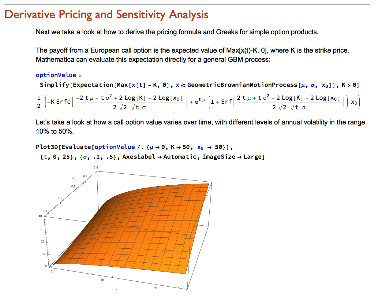
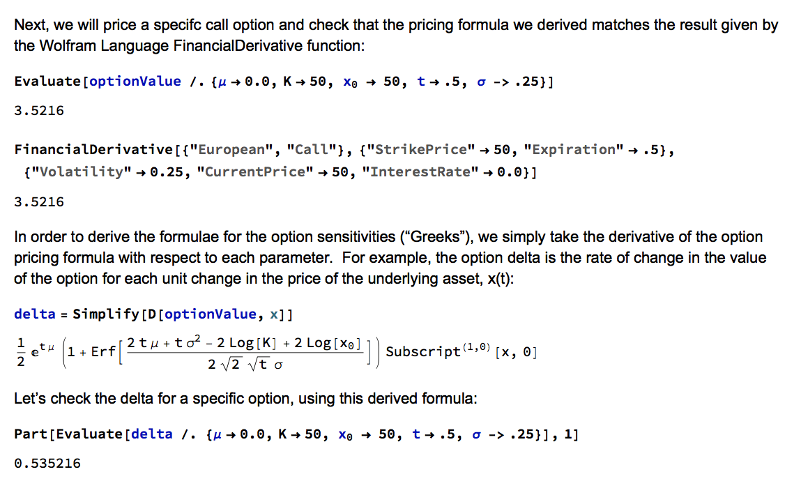
The advantages of this approach are considerable. The capabilities of the language make it easy to provide interactive examples to illustrate theoretical concepts and develop the student’s understanding of them through experimentation. Furthermore, the student is not limited merely to learning and applying complex formulae for derivative pricing and risk, but can fairly easily derive the results for themselves. As a consequence, a course in stochastic calculus taught using Mathematica can be broader in scope and go deeper into the theory than is typically the case, while at the same time reinforcing understanding and learning by practical example and experimentation.

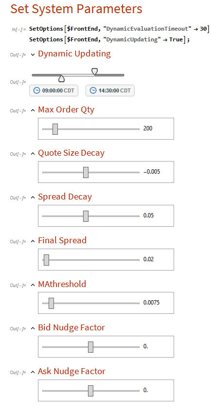
This algorithm builds on the research by Stoikova and Avelleneda in their 2009 paper “High Frequency Trading in a Limit Order Book“, 2009 and extends the basic algorithm in several ways:
The algorithm is implemented in Mathematica, and can be compiled to create dlls callable from with a C++ or Python application.
The application makes use of the MATH-TWS library to connect to the Interactive Brokers TWS or Gateway platform via the C++ api. MATH-TWS is used to create orders, manage positions and track account balances & P&L.

Happy New Year to my readers.
I recently pitched a consulting project that entailed building a stock screener that would apply both fundamental and technical criteria to identity a universe of candidate stocks across world-wide equity markets.
Here is how I approached the task:

At long last, it’s here!
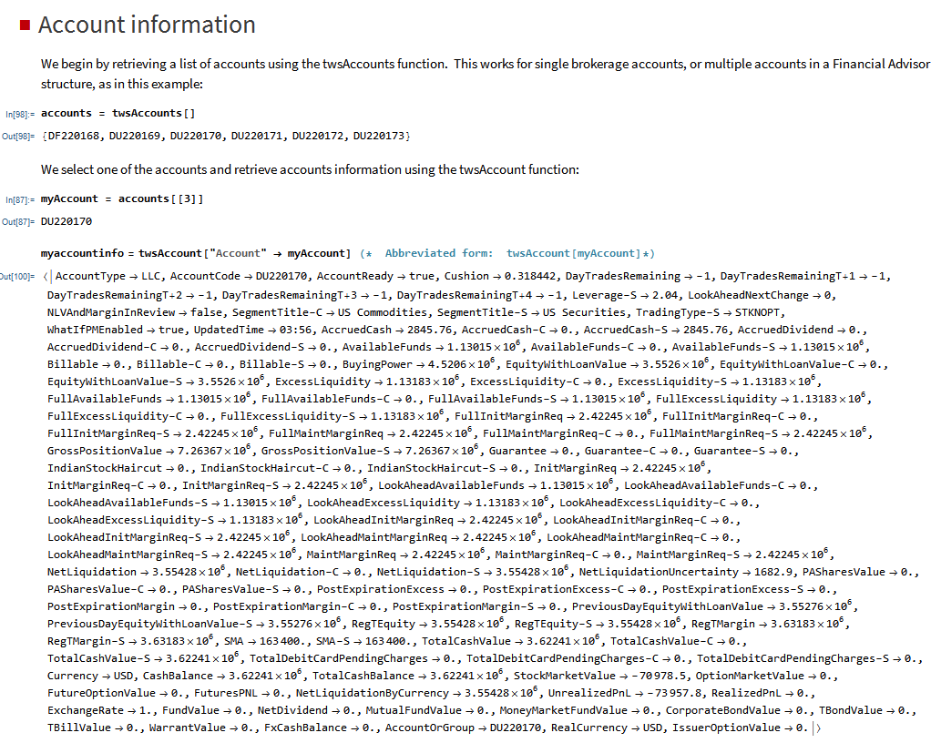
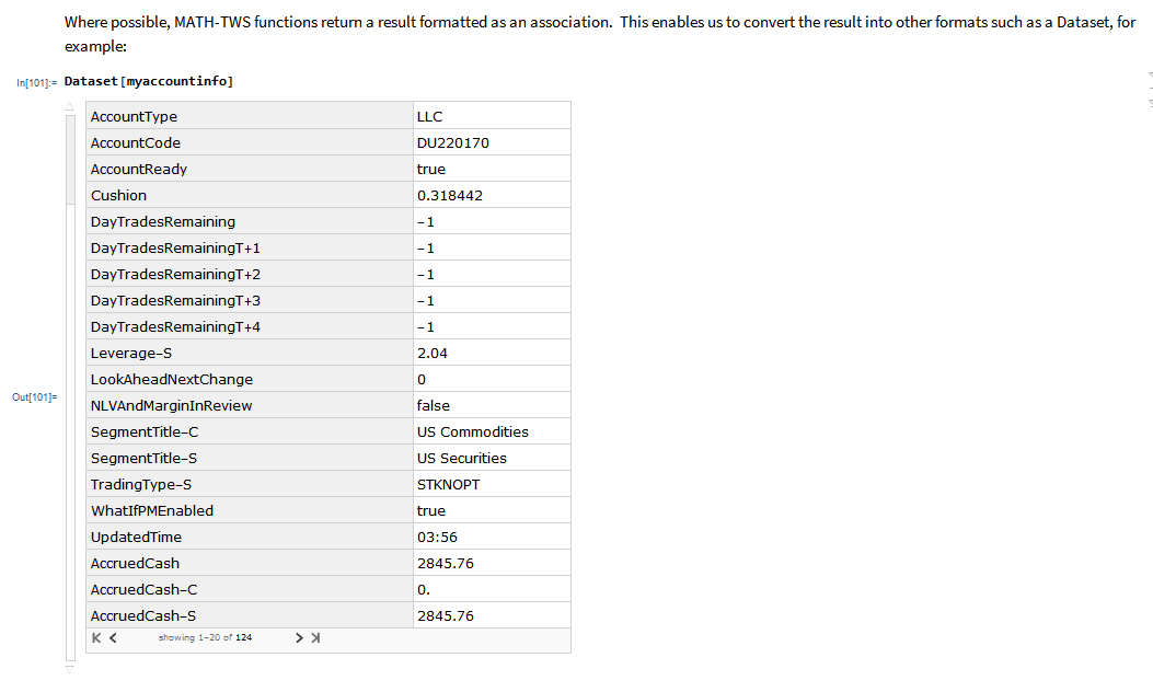
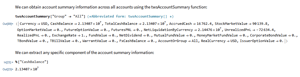
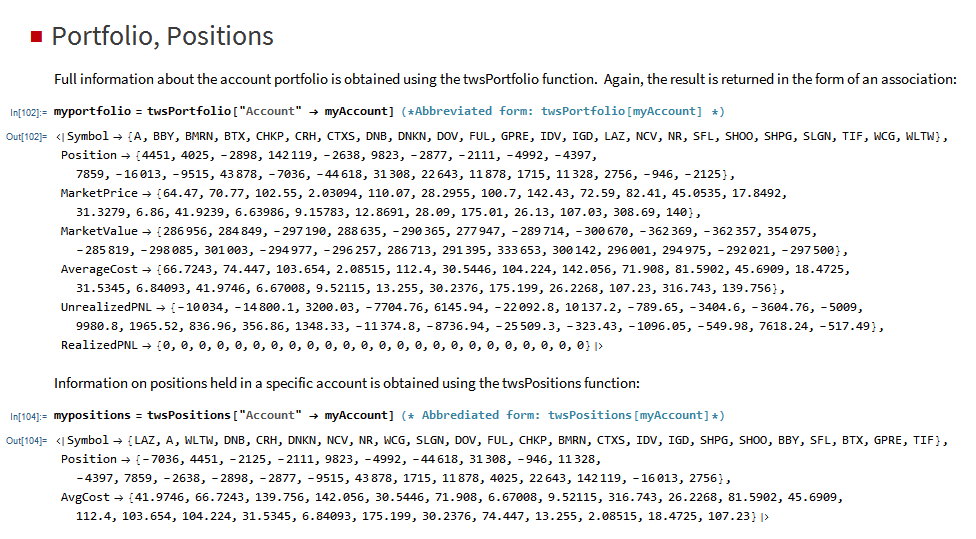
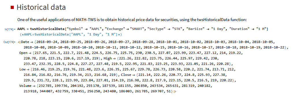
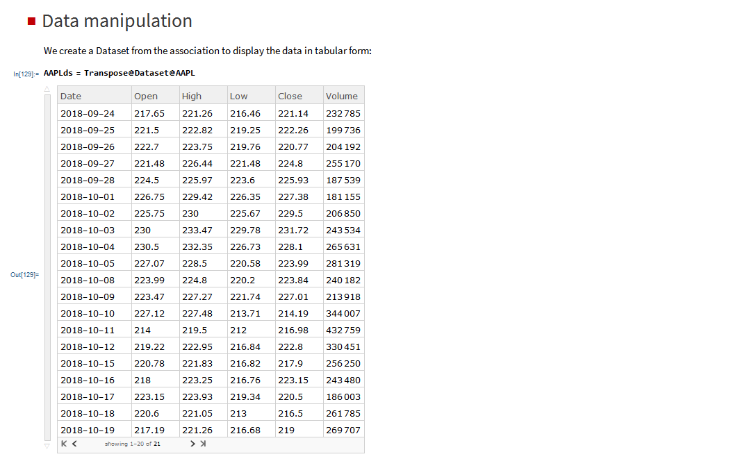
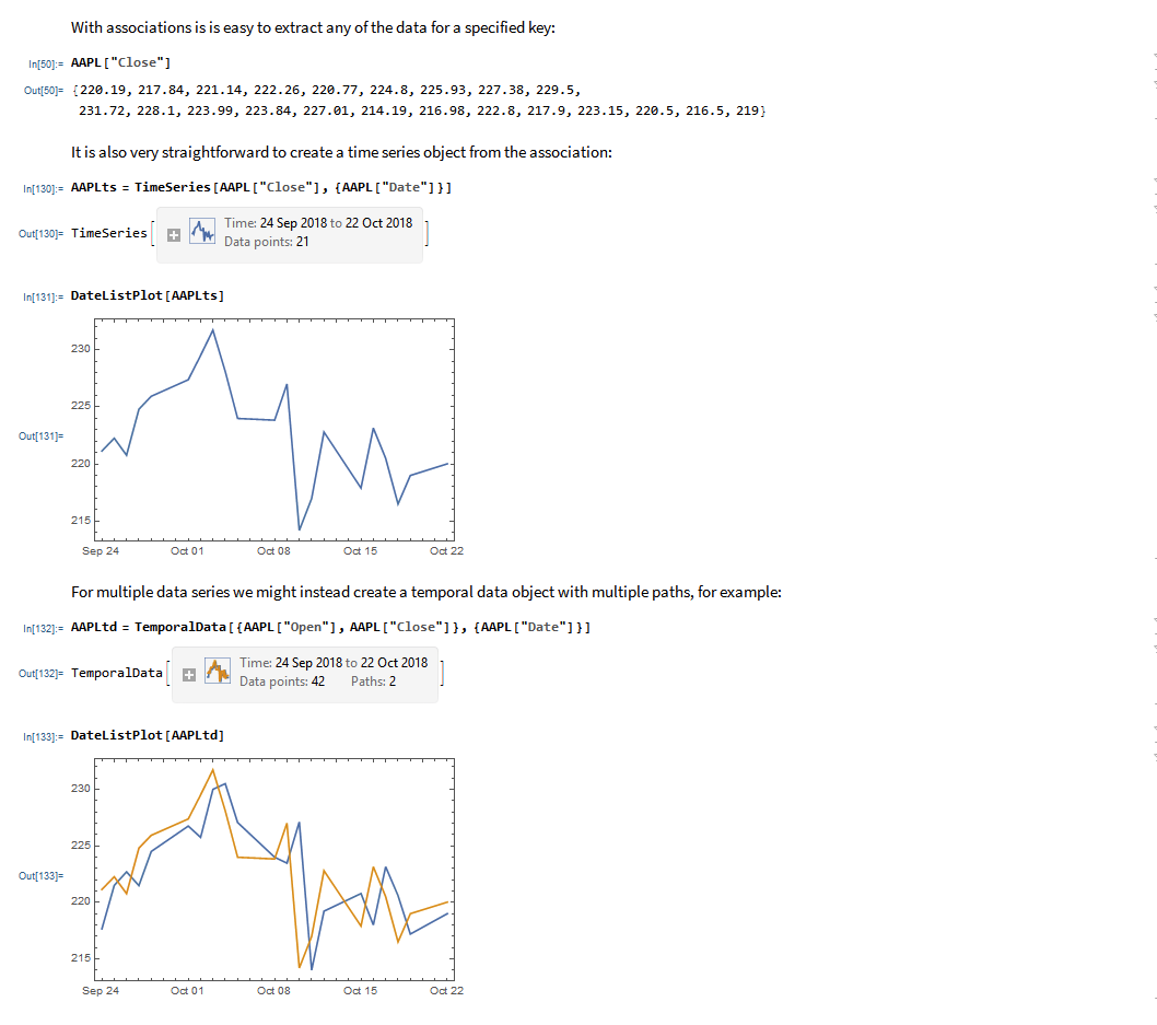
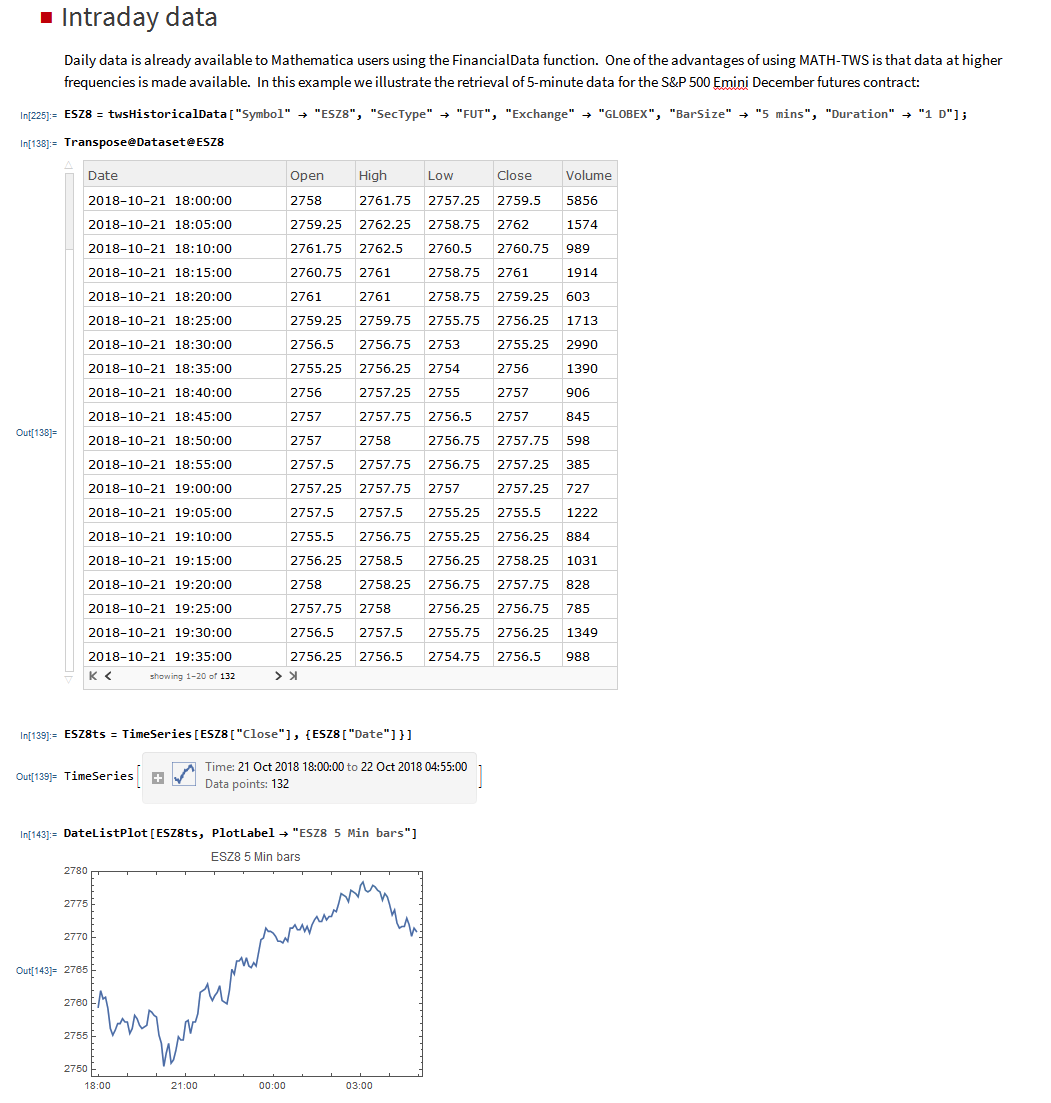
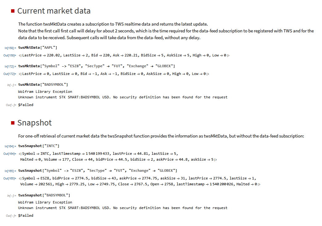
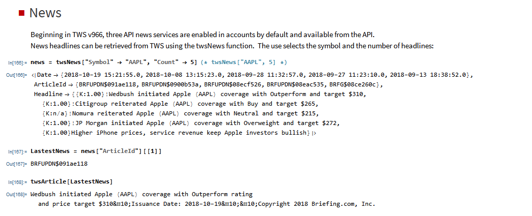
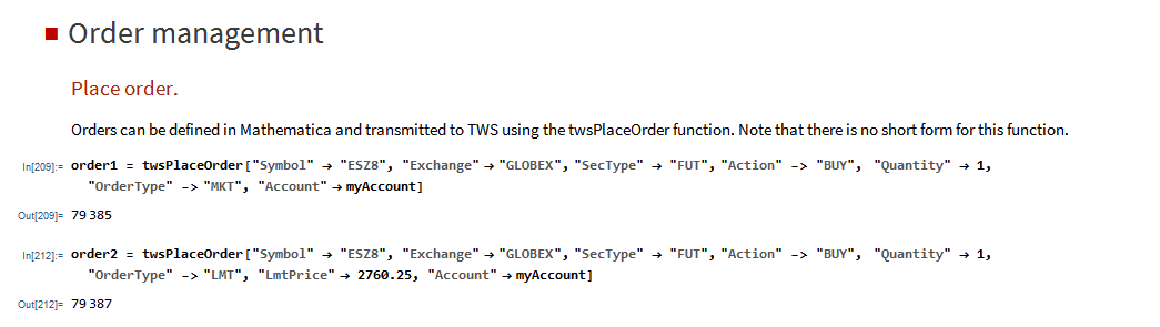
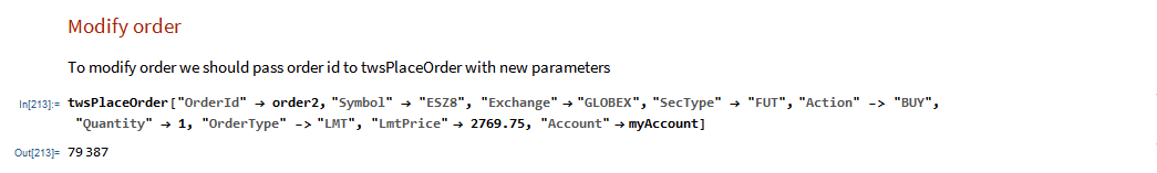
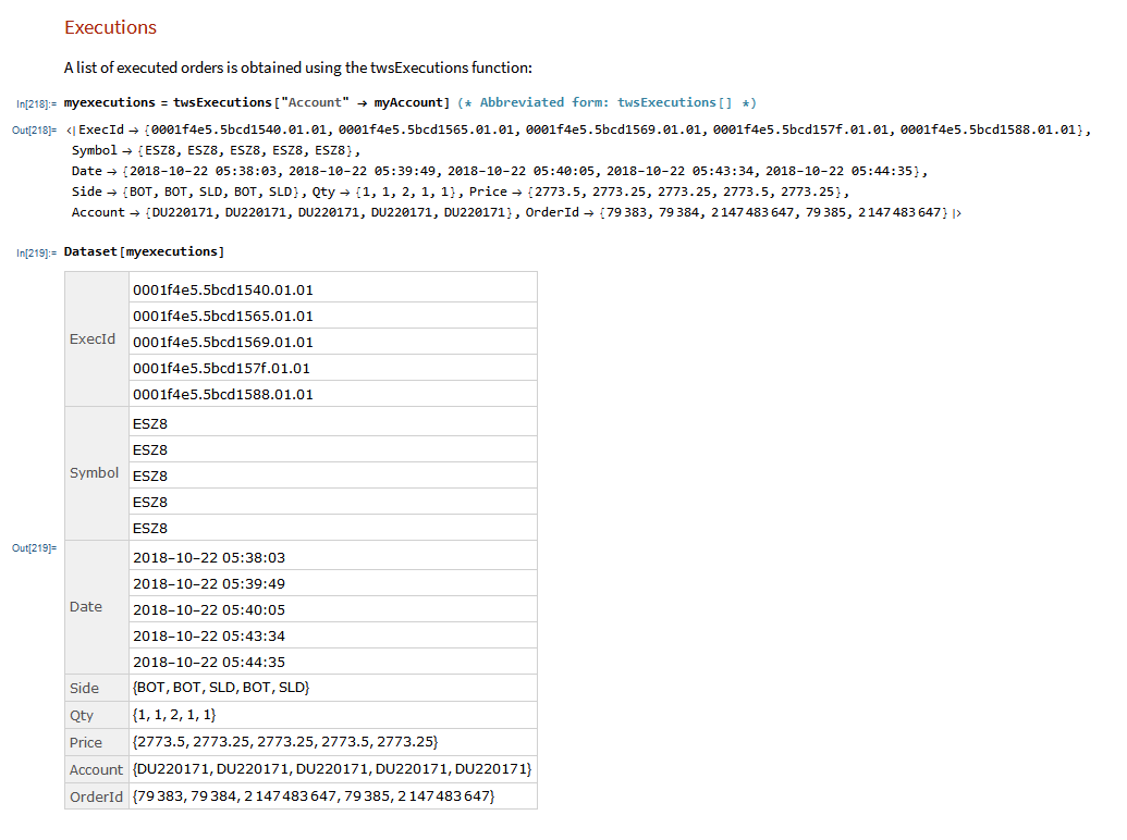
MATH-TWS is a new Mathematica package that connects Wolfram Mathematica to the Interactive Brokers TWS platform via the C++ API. It enables the user to retrieve information from TWS on accounts, portfolios and positions, as well as historical and real-time market data. MATH-TWS also enables the user to place and amend orders and obtain execution confirmations from Mathematica.
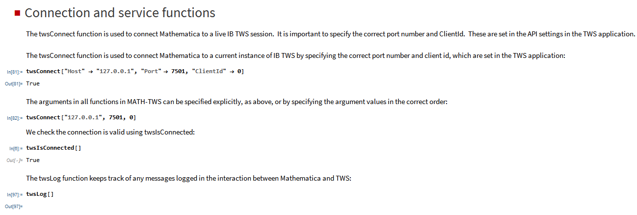
In the following sections we will illustrate the functionality of the MATH-TWS package using the full functional form and show the abbreviated equivalent form in comments.

I have wanted a way to connect Wolfram Mathematica to Interactive Brokers’ Trader Workstation for the longest time. Now that it is finally available with MATH-TWS I am excited by the possibilities for Mathematica users.
The first release of MATH-TWS will be available within a couple of weeks. Anyone interested in licensing a copy should email algorithmicexecution@gmail.com with MATH-TWS in the subject line.
Towards the end of last year I wrote a post (see here) about the advent of modern programming languages, including the JIT compiled Julia and visual programming language ADL from Trading Technologies. My conclusion (based on a not very scientific sample) was that we appear to be at the tipping point, where the speed of newer, high level languages languages is approaching that of the fastest compiled languages like C/C++.
Now comes a formal academic study of the topic in A Comparison of Programming Languages in Economics, Aruoba and Fernandez-Villaverde, 2014. Using the neoclassical growth model, the authors conduct a benchmark test in C++11, Fortran 2008, Java, Julia, Python, Matlab, Mathematica, and R, implementing the same algorithm, value function
iteration with grid search, in each of the languages. They report the execution times of the codes in a Mac and in a Windows computer and briefly comment on the strengths and weaknesses of each language.
The conclusions from the study mirror my own thoughts on the subject very closely. The authors find that:
C++ still represents the benchmark for speed, but not by much. It is barely faster than the old stalwart, Fortran, and only 1.5 – 3 times faster than up-and-coming rivals amongst the higher level languages (especially when you allow for hybrid programming to speed up the slowest algorithms).
So, as regards developing financial models and trading systems, my questions are (as before):
When you reach a point where a high level language like Matlab is only around 1.5x – 2x slower than C++, you really have to question whether the latter is an appropriate choice. Yes, of course, in mission-critical applications where you need access to the hardware layer for speed purposes, C++ is the way to go. But for so many applications, that just isn’t the case.
What matters, far, far more, are the months of costly and laborious programming effort that is often required to reproduce basic functionality that is already embedded in higher level languages like Matlab or Mathematica. Not only that, but the end result of a C++ /Java development effort is likely to be notoriously inflexible by comparison. That’s a huge drawback. Rarely, if ever, does a piece of research translate flawlessly into production – it requires one to iterate towards a final solution, often making significant changes to the design of the system in the light of practical experience.
If I had to guess, based on my experience, I would say that 80% or more of development tasks in quantitative research and trading would produce a superior result if preference was given to using a higher level language for the initial development. When the system is sufficiently stable to put into production, you simply create a hybrid application by recoding any mission-critical components for which speed is an issue in C++.
Finally, where does that leave my beloved Mathematica? To be fair, while you don’t have the joys of strong typing to contend with, Mathematica’s syntax is just as demanding and uncompromising as C++ – a missed comma or incorrectly placed bracket is just as critical. But, the point is, while in C++ the syntactical rigor is just annoying, in Mathematica it’s worth putting up with because the productivity is so much greater. A competent programmer can produce, in a single line of Mathematica code, a program that would require hundreds, if not thousands of lines of C++ code to accomplish. Sure, he might get the syntax wrong at first: but it’s only a single line of code and the interactive gui interface makes debugging very simple.
That said, while Mathematica can be very tedious to use for procedural programming, it excels in three areas:
1. Symbolic programming. Anything involving mathematical symbols and equations – Mathematica is #1
2. User interface. In Mathematica, it is trivial to build a sophisticated, dynamic gui in no time at all, again, often in 1-2 lines of code
3. Functional programming. Anything that can be thought of as a function, Mathematica handles extremely well. We are not talking about finding a square root here: I mean extremely complex functions that, again, might take hundreds of lines of code in another language.
It is also worth pointing out that Mathematica comes supplied with functionality that Matlab provides only through numerous, costly add-on packages.
CONCLUSION
Before I allow a development team to start mindlessly coding up a system in Java or C++, I want to hear their reasons why they aren’t going to do it 10x faster in another, higher level language. “We always use C++/Java for production” is not a reason. Specifically, which parts of the system require the additional 1.5x speed-up, and why can’t they be coded as dlls (Matlab mex functions)?
Finally, on a cost-benefit basis, ask yourself how much you might benefit if the months and tens (or hundreds) of thousands of dollars wasted on developing in C++ were instead spent on researching and developing new trading ideas.