In a previous blog post I mentioned the VVIX/VIX Ratio, which is measured as the ratio of the CBOE VVIX Index to the VIX Index. The former measures the volatility of the VIX, or the volatility of volatility.
http://jonathankinlay.com/2017/07/market-stress-test-signals-danger-ahead/
A follow-up article in ZeroHedge shortly afterwards pointed out that the VVIX/VIX ratio had reached record highs, prompting Goldman Sachs analyst Ian Wright to comment that this could signal the ending of the current low-volatility regime:
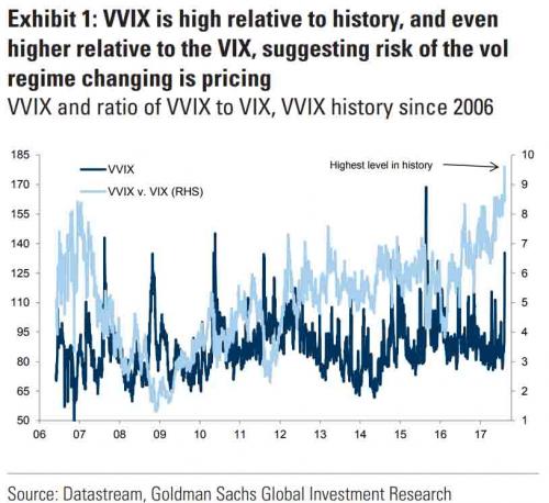
A linkedIn reader pointed out that individual stock volatility was currently quite high and when selling index volatility one is effectively selling stock correlations, which had now reached historically low levels. I concurred:
What’s driving the low vol regime is the exceptionally low level of cross-sectional correlations. And, as correlations tighten, index vol will rise. Worse, we are likely to see a feedback loop – higher vol leading to higher correlations, further accelerating the rise in index vol. So there is a second order, Gamma effect going on. We see that is the very high levels of the VVIX index, which shot up to 130 last week. The all-time high in the VVIX prior to Aug 2015 was around 120. The intra-day high in Aug 2015 reached 225. I’m guessing it will get back up there at some point, possibly this year.
As there appears to be some interest in the subject I decided to add a further blog post looking a little further into the relationship between volatility and correlation. To gain some additional insight we are going to make use of the CBOE implied correlation indices. The CBOE web site explains:
Using SPX options prices, together with the prices of options on the 50 largest stocks in the S&P 500 Index, the CBOE S&P 500 Implied Correlation Indexes offers insight into the relative cost of SPX options compared to the price of options on individual stocks that comprise the S&P 500.
- CBOE calculates and disseminates two indexes tied to two different maturities, usually one year and two years out. The index values are published every 15 seconds throughout the trading day.
- Both are measures of the expected average correlation of price returns of S&P 500 Index components, implied through SPX option prices and prices of single-stock options on the 50 largest components of the SPX.
Dispersion Trading
One application is dispersion trading, which the CBOE site does a good job of summarizing:
The CBOE S&P 500 Implied Correlation Indexes may be used to provide trading signals for a strategy known as volatility dispersion (or correlation) trading. For example, a long volatility dispersion trade is characterized by selling at-the-money index option straddles and purchasing at-the-money straddles in options on index components. One interpretation of this strategy is that when implied correlation is high, index option premiums are rich relative to single-stock options. Therefore, it may be profitable to sell the rich index options and buy the relatively inexpensive equity options.
The VIX Index and the Implied Correlation Indices
Again, the CBOE web site is worth quoting:
The CBOE S&P 500 Implied Correlation Indexes measure changes in the relative premium between index options and single-stock options. A single stock’s volatility level is driven by factors that are different from what drives the volatility of an Index (which is a basket of stocks). The implied volatility of a single-stock option simply reflects the market’s expectation of the future volatility of that stock’s price returns. Similarly, the implied volatility of an index option reflects the market’s expectation of the future volatility of that index’s price returns. However, index volatility is driven by a combination of two factors: the individual volatilities of index components and the correlation of index component price returns.
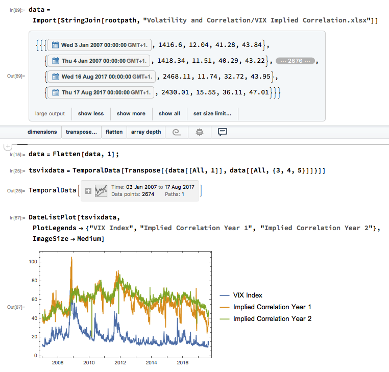
Let’s dig into this analytically. We first download and plot the daily for the VIX and Correlation Indices from the CBOE web site, from which it is evident that all three series are highly correlated:
An inspection reveals significant correlations between the VIX index and the two implied correlation indices, which are themselves highly correlated. The S&P 500 Index is, of course, negatively correlated with all three indices:
Modeling Volatility-Correlation
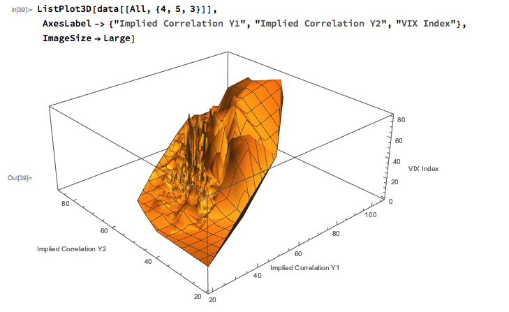
The response surface that describes the relationship between the VIX index and the two implied correlation indices is locally very irregular, but the slope of the surface is generally positive, as we would expect, since the level of VIX correlates positively with that of the two correlation indices.
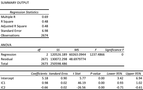
The most straightforward approach is to use a simple linear regression specification to model the VIX level as a function of the two correlation indices. We create a VIX Model Surface object using this specification with the Mathematica Predict function: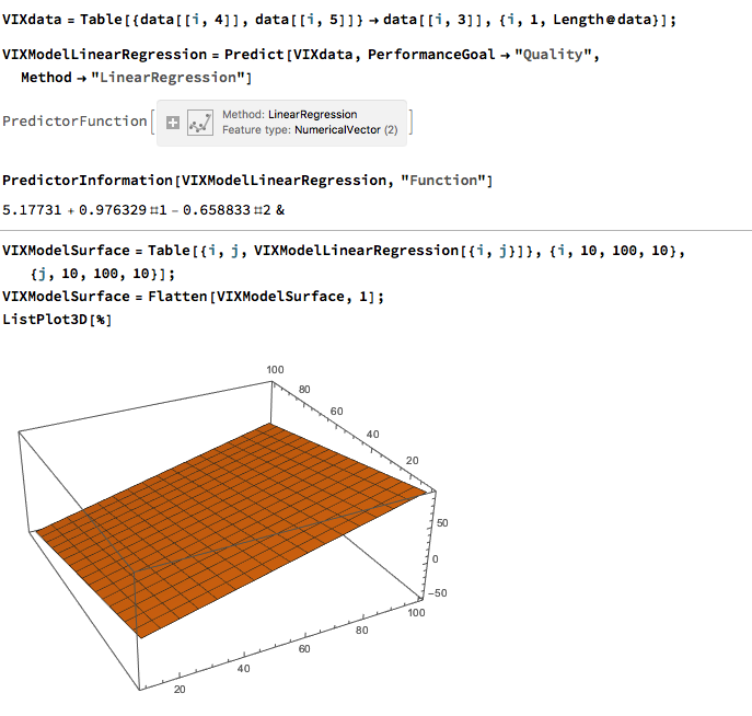 The linear model does quite a good job of capturing the positive gradient of the response surface, and in fact has a considerable amount of explanatory power, accounting for a little under half the variance in the level of the VIX index:
However, there are limitations. To begin with, the assumption of independence between the explanatory variables, the correlation indices, clearly does not hold. In cases such as this, where explanatory variables are multicolinear, we are unable to draw inferences about the explanatory power of individual regressors, even though the model as a whole may be highly statistically significant, as here.
Secondly, a linear regression model is not going to capture non-linearities in the volatility-correlation relationship that are evident in the surface plot. This is confirmed by a comparison plot, which shows that the regression model underestimates the VIX level for both low and high values of the index:
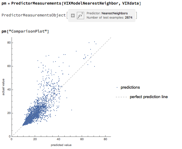
We can achieve a better outcome using a machine learning algorithm such as nearest neighbor, which is able to account for non-linearities in the response surface:
The comparison plot shows a much closer correspondence between actual and predicted values of the VIX index, even though there is evidence of some remaining heteroscedasticity in the model residuals:
Conclusion
A useful way to think about index volatility is as a two dimensional process, with time-series volatility measured on one dimension and dispersion (cross-sectional volatility, the inverse of correlation) measured on the second. The two factors are correlated and, as we have shown here, interact in a complicated, non-linear way.
The low levels of index volatility we have seen in recent months result, not from low levels of volatility in component stocks, but in the historically low levels of correlation (high levels of dispersion) in the underlying stock returns processes. As correlations begin to revert to historical averages, the impact will be felt in an upsurge in index volatility, compounded by the non-linear interaction between the two factors.


